Spatial Poisson process

In statistics and probability theory the spatial Poisson process (SPP) is a multidimensional generalization of the Poisson process, which can be described as a counting process where the number of points (events) in disjoint intervals are independent and have a Poisson distribution. Similarly, one can think of "points" being scattered over a $d$ -dimensional space in some random manner and of the spatial Poisson process as counting the number of points in a given set. It is also common to speak of a Poisson point process instead of a SPP.

Definition

Usually, the SPP is considered on the Euclidean space $\mathbb{R}^d$ where $d \geq 1$ . Firstly it is needed to give some technical definitions. Likewise to the one-dimensional case a realization of a SPP on $\mathbb{R}^d$ is assumed to be a countable subset $\Pi$ of $\mathbb{R}^d$ . Thus, $\Pi$ can be seen as a countable set of points. The distribution of $\Pi$ through the number $|\Pi \cap A |$ of its points lying in a subset $A \subset \mathbb{R}^d$ is going to be examined. It is assumed, that there is a well defined notion of the "volume" of $A$ . More Specifically, it is assumed that $A\in \mathcal{B}^d$ , in other words $A$ is in the Borel- $\sigma$ algebra. Writing $|A|$ we mean the volume given by the Lebesgue measure of the Borel set $A$ .^[1]

More generally it is possible to consider a state space $S\not\subset\mathbb{R}^d$ in which the points of a Poisson process sit. Though, it is naturally assumed that $S$ is a measurable space and that its measurable sets form a $\sigma$ . It is also possible to define the SPP with a general measure $\mu$ instead of using the Lebesgue measure. In that case $|\Pi \cap A |$ is replaced by $\mu(\Pi \cap A )$ . ^[2]

It is common to distinguish between the homogeneous and inhomogeneous case:

Homogeneous spatial Poisson process

The random countable subset $\Pi$ of $\mathbb{R}^d$ is called a homogeneous spatial Poisson process with (constant) intensity $\lambda$ if, for all $A \in \mathcal{B}^d$ , the random variables $N(A):=|\Pi \cap A|$ satisfy:^[1]

$N(A)$ has the Poisson distribution with parameter $\lambda|A|$ , and
if $A_1,A_2,\ldots,A_n$ are disjoint sets in $\mathcal{B}^d$ , then $N(A_1), N(A_2),\ldots , N(A_n)$ are independent random variables.

The counting process $N$ is commonly referred to be itself a Poisson process if it satisfies 1. and 2. above. The special case when $\lambda>0$ and $|A| = \infty$ , the situation is interpreted as $\mathbb{P}(|\Pi \cap A |=\infty)=1$ .

Inhomogeneous spatial Poisson process

Roughly speaking, the inhomogeneous case differs from the homogeneous case by the intensity $\lambda$ , which is not constant anymore. As indicated above, it is useful to have a definition of a Poisson process with other measures than Lebesgue measure. In order to get another measure $\Lambda(A)$ than $|A|$ the Euclidean element $\lambda d \textbf{x}$ is replaced by the element $\lambda(\textbf{x})d \textbf{x}$ . As a consequence the definition follows $\Lambda(A):=\int_A \lambda(\textbf{x}) \, d \textbf{x},\quad A\in \mathcal{B}^d.$

That leads to the following
Definition^[1] Let $\lambda: \mathbb{R}^d\to \mathbb{R}$ be a non-negative measurable function such that $\Lambda(A)<\infty$ for all bounded $A$ . The random countable subset $\Pi\subset \mathbb{R}^d$ is called inhomogeneous spatial Poisson process with intensity function $\lambda$ if, for all $\mathcal{B}^d$ , the random variables $N(A)=|\Pi\cap A|$ satisfy:

$N(A)$ has the Poisson distribution with parameter $\Lambda(A)$ , and
if $A_1,A_2,\ldots,A_n$ are disjoint sets in $\mathcal{B}^d$ , then $N(A_1), N(A_2),\ldots , N(A_n)$ are independent random variables.

The function $\Lambda(A), A\in \mathcal{B}^d$ is often called the mean measure of the process $\Pi$ .

Examples

Besides the application of the Poisson process in one dimension, there are many examples in two and higher dimensions. Modeling with a spatial Poisson process can be done in the following situations:^[1]^[3]

The distribution of stars in a galaxy or of galaxies in the universe,
Positions of animals in their habitat,
The locations of active sites in a chemical reaction or of the weeds in your lawn,
Defects on a surface or in a volume in reliability engineering.
Positionally resolved photo-electron events on a photo-cathode focal plane array.

Even when a Poisson process is not a perfect description of such a system, it can provide a relatively simple yardstick against which to measure the improvements which may be offered by more sophisticated but often less tractable models.

Mathematical properties

Many properties known from the Poisson Process hold also true in the multidimensional process. The Poisson point process is also characterized by the single parameter $\lambda$ . It is a simple, stationary point process with mean measure $\lambda$ . ^[2]

Equivalent formulation

It can be shown, that because of the two essential conditions the distribution of the spatial Poisson process is given by^[2]

\mathbb{P}(N(A_i) = k_i, 1 \leq i \leq n) = \dfrac{(\lambda A_1)^{k_1}}{k_1!}\cdot e^{-\lambda |A_1|}\cdots \dfrac{(\lambda A_n)^{k_n}}{k_n!}\cdot e^{-\lambda |A_n|},

for any disjoint bounded subsets $A_1,...,A_n$ and non-negative integers $k_1,\ldots,k_n$ .

Derivation from physically postulates

Using the law of rare events the Poisson process can be concluded by certain physically plausible postulates.^[3] Let $N(A)$ be a random point process fulfilling these postulates, then $N(A)$ is a homogeneous Poisson Point Process with intensity $\lambda$ derived from the postulates and the distribution is given as above in the Equivalent Formulation. Namely the four postulates are:

The possible values for $N(A)$ are the nonnegative integers $\{0,1,2,\ldots\}$ and $0<\mathbb{P}(N(A)=0)<1$ if $0<|A|< \infty$ .
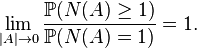
The probability distribution of $N(A)$ depends on the set $A$ only through its size (length, area, or volume) $|A|$ , with the further property that $0<\mathbb{P}(N(A) \geq 1)=\lambda|A|+o(|A|)$ as $|A| \downarrow 0.$
For $m\geq 2,$ if $A_1,\ldots,A_m$ are disjoint regions, then $N(A_1),N(A_2),\ldots,N(A_m)$ are independent random variables and $N(A_1 \cup A_2 \cup \cdots \cup A_m)=N(A_1)+N(A_2)+\cdots + N(A_m).$
$\lim\limits_{|A|\to 0} \dfrac{\mathbb{P}(N(A)\geq 1)}{\mathbb{P}(N(A)=1)}=1.$

While postulate 1 excludes extreme or trivial cases, the second one asserts that the probability distribution of $N(A)$ does depend only on the size of $A$ , not on the shape or location. Thirdly it is postulated, that disjoint regions are independent regarding the outcome of the process. Finally, postulate 4 requires that there cannot be tow points occupying the same location.

Distribution of n points in a given set

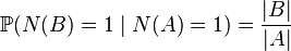
We are interested in the distribution of a point from which is supposed to be contained in a region $A$ with positive size $|A|>0$ . In other words: $N(A)=1$ . The question where the point can be found in $A$ is answered by a uniform distribution:^[3]

\mathbb{P}(N(B)=1 \mid N(A)=1)= \dfrac{|B|}{|A|}

for any set

B\subset A

Consider again a region with positive size $|A|>0$ , and suppose now it is known that $A$ contains exactly $n$ points. Then, these points are independent and uniformly distributed in $A$ in the sense that for any disjoint partition $A_1,\ldots,A_m$ of $A$ , and any positive integers $k_i$ , where $k_1+\cdots + k_m=n$ , we have

\mathbb{P}(N(A_1)=k_1,\ldots,N(A_m)=k_m \mid N(A)=n)= \dfrac{n!}{k_1!\cdots k_m!}\left(\dfrac{|A_1|}{|A|}\right)^{k_1}\cdots \left(\dfrac{|A_m|}{|A|}\right)^{k_m}.

Thus, the conditional distribution follows a multinomial distribution.^[3]

Other properties

The union of two independent SPP is again a spatial Poisson process:
Superposition Theorem^[1] Let $\Pi'$ and $\Pi''$ be independent Poisson processes on $\mathbb{R}^d$ with respective intensity functions $\lambda'$ and $\lambda''$ . The set $\Pi=\Pi'\cup\Pi''$ is a Poisson process with intensity function $\lambda=\lambda'+\lambda''$ .
The theorem can be generalized to the union of more than two processes.

There exist a complementary version to the superposition theorem:
Colouring theorem^[1] Let $\Pi$ be a non-homogeneous Poisson process on $\mathbb{R}^d$ with intensity function $\lambda(\textbf{x})$ . We colour the points of $\Pi$ in the following way. A point of $\Pi$ at position x is coloured green with probability $\gamma(\textbf{x})$ ; otherwise it is coloured scarlet (with probability $\sigma(\textbf{x})=1-\gamma(\textbf{x})$ ). Points are coloured independently of one another. Let $\Gamma$ and $\Sigma$ be the sets of points coloured green and scarlet, respectively. Then $\Gamma$ and $\Sigma$ are independent Poisson processes with respective intensity functions $\gamma(\textbf{x})\lambda(\textbf{x})$ and $\sigma(\textbf{x})\lambda(\textbf{x})$ .

Generalization

The Spatial Poisson Process is a very common example of a Point process.

References

↑ 1.0 1.1 1.2 1.3 1.4 1.5 G. R. Grimmett, D. Stirzaker, Probability and Random Processes , Oxford University Press, Third Edition 2001, pages 281–292
↑ 2.0 2.1 2.2 J. F. C. Kingman, Poisson Processes, Oxford Studies in Probability, Oxford University Press New York, 1993, pages 11–25
↑ 3.0 3.1 3.2 3.3 Mark A. Pinsky, Samuel Karlin, An Introduction to Stochastic Modeling , Elsevier, Fourth Edition 2011, pages 259–263