Solvency cone
The solvency cone is a concept used in financial mathematics which models the possible trades in the financial market. This is of particular interest to markets with transaction costs. Specifically, it is the convex cone of portfolios that can be exchanged to portfolios of non-negative components (including paying of any transaction costs).
Mathematically
If given a bid-ask matrix  for
for  assets such that
  and
and  is the number of assets which with any non-negative quantity of them can be "discarded" (traditionally
  ). Then the solvency cone
  is the convex cone spanned by the unit vectors
  and the vectors
  .[1]
.[1]
Definition
A solvency cone  is any closed convex cone such that
  and
and  .[2]
.[2]
Uses
A process of (random) solvency cones  is a model of a financial market. This is sometimes called a market process.
The negative of a solvency cone is the set of portfolios that can be obtained starting from the zero portfolio. This is intimately related to self-financing portfolios.
The dual cone of the solvency cone ( ) are the set of prices which would define a friction-less pricing system for the assets that is consistent with the market. This is also called a consistent pricing system.[1]
Examples


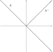
Assume there are 2 assets, A and M with 1 to 1 exchange possible.
Frictionless Market
In a frictionless market, we can obviously make (1A,-1M) and (-1A,1M) into non-negative portfolios, therefore  . Note that (1,1) is the "price vector."
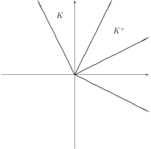
With Transaction Costs
Assume further that there is 50% transaction costs for each deal. This means that (1A,-1M) and (-1A,1M) cannot be exchanged into non-negative portfolios. But, (2A,-1M) and (-1A,2M) can be traded into non-negative portfolios. It can be seen that  .
.
The dual cone of prices is thus easiest to see in terms of prices of A in terms of M (and similarly done for price of M in terms of A):
- someone offers 1A for tM:
 therefore there is arbitrage if
- someone offers tM for 1A:
 therefore there is arbitrage if
Notes
If a solvency cone  :
:
- contains a line, then there is an exchange possible without transaction costs.
-
 , then there is no possible exchange, i.e. the market is completely illiquid.
References
- ↑ 1.0 1.1 Schachermayer, Walter (November 15, 2002). "The Fundamental Theorem of Asset Pricing under Proportional Transaction Costs in Finite Discrete Time".
- ↑ Hamel, A. H.; Heyde, F. (2010). "Duality for Set-Valued Measures of Risk" (pdf). SIAM Journal on Financial Mathematics 1 (1): 66–95. doi:10.1137/080743494. Retrieved August 17, 2012.