Slope field

The slope field of dy/dx=x²-x-2, with the blue, red, and turquoise lines being (x³/3)-(x²/2)-2x+4, (x³/3)-(x²/2)-2x, and (x³/3)-(x²/2)-2x-4, respectively.

In mathematics, a slope field (or direction field) is a graphical representation of the solutions of a first-order differential equation. It is useful because it can be created without solving the differential equation analytically. The representation may be used to qualitatively visualize solutions, or to numerically approximate them.

Definition

Standard case

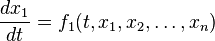
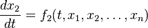
The slope field is traditionally defined for the following type of differential equations

y'=f(x,y)

It can be viewed as a creative way to plot a real-valued function of two real variables $f(x,y)$ as a planar picture. Specifically, for a given pair $x,y$ , a vector with the components $[1, f(x,y)]$ is drawn at the point $x,y$ on the $x,y$ -plane. Sometimes, the vector $[1, f(x,y)]$ is normalized to make the plot better looking for a human eye. A set of pairs $x,y$ making a rectangular grid is typically used for the drawing.

An Isocline (a series of lines with the same slope) is often used to supplement the slope field. In an equation of the form $y'=f(x,y)$ , the isocline is a line in the $x,y$ -plane plane obtained by setting $f(x,y)$ equal to a constant.

General case of a system of differential equations

Given a system of differential equations,

\frac{dx_1}{dt}=f_1(t,x_1,x_2,\ldots,x_n)

\frac{dx_2}{dt}=f_2(t,x_1,x_2,\ldots,x_n)

\vdots

\frac{dx_n}{dt}=f_n(t,x_1,x_2,\ldots,x_n)

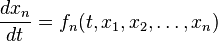
the slope field is an array of slope marks in the phase space (in any number of dimensions depending on the number of relevant variables; for example, two in the case of a first-order linear ODE, as seen to the right). Each slope mark is centered at a point $(t,x_1,x_2,\ldots,x_n)$ and is parallel to the vector

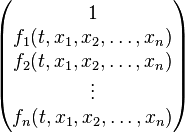\begin{pmatrix} 1 \\ f_1(t,x_1,x_2,\ldots,x_n) \\ f_2(t,x_1,x_2,\ldots,x_n) \\ \vdots \\ f_n(t,x_1,x_2,\ldots,x_n) \end{pmatrix}

The number, position, and length of the slope marks can be arbitrary. The positions are usually chosen such that the points $(t,x_1,x_2,\ldots,x_n)$ make a uniform grid. The standard case, described above, represents $n=1$ . The general case of the slope field for systems of differential equations is not easy to visualize for $n>2$ .

General application

With computers, complicated slope fields can be quickly made without tedium, and so an only recently practical application is to use them merely to get the feel for what a solution should be before an explicit general solution is sought. Of course, computers can also just solve for one, if it exists.

If there is no explicit general solution, computers can use slope fields (even if they aren’t shown) to numerically find graphical solutions. Examples of such routines are Euler's method, or better, the Runge-Kutta methods.

Software for plotting slope fields

Different software packages can plot slope fields.

Example code in GNU Octave/MATLAB

Ffun = @(X,Y)X.*Y;               % function f(x,y)=xy
[X,Y]=meshgrid(-2:.3:2,-2:.3:2); % choose the plot sizes
DY=Ffun(X,Y); DX=ones(size(DY)); % generate the plot values 
quiver(X,Y,DX,DY);               % plot the direction field
hold on;
contour(X,Y,DY,[-6 -2 -1 0 1 2 6]); %add the isoclines
title('Slope field and isoclines for f(x,y)=xy')

Alternate example code in GNU Octave/MATLAB

funn = @(x,y)y-x;                % function f(x,y)=y-x
[x,y]=meshgrid(-2:0.5:2);        % intervals for x and y
slopes=funn(x,y);                % matrix of slopes
dy=slopes./sqrt(1+slopes.^2);    % normalize the line element...
dx=sqrt(1-dy.^2);                % ...magnitudes for dy and dx 
quiver(x,y,dx,dy);               % plot the direction field

Example code for Maxima

/* field for y'=xy (click on a point to get an integral curve) */
plotdf( x*y, [x,-2,2], [y,-2,2]);

Examples

y' = xy
Slope field
Integral curves
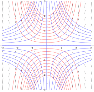
Isoclines (blue), slope field (black), and some solution curves (red)

References

Blanchard, Paul; Devaney, Robert L.; and Hall, Glen R. (2002). Differential Equations (2nd ed.). Brooks/Cole: Thompson Learning. ISBN 0-534-38514-1