Signorini problem

The Signorini problem is an elastostatics problem in linear elasticity: it consists in finding the elastic equilibrium configuration of an anisotropic non-homogeneous elastic body, resting on a rigid frictionless surface and subject only to its mass forces. The name was coined by Gaetano Fichera to honour his teacher, Antonio Signorini: the original name coined by him is problem with ambiguous boundary conditions.

History

The classical Signorini problem: what will be the equilibrium configuration of the orange spherically shaped elastic body resting on the blue rigid frictionless plane?

The problem was posed by Antonio Signorini during a course taught at the Istituto Nazionale di Alta Matematica in 1959, later published as the paper Signorini 1959, expanding a previous short exposition he gave in a note published in 1933. According to Signorini (1959, p. 128) himself, he called it problem with ambiguous boundary conditions^[1] since there are two alternative sets of boundary conditions the solution must satisfy on any given contact point, involving not only equalities but also inequalities, but it is not a priori known what of the two sets is satisfied for each point: he asked to determine if the problem is well-posed or not in a physical sense, i.e. if its solution exists and is unique or not, inviting young analysts to study the problem.^[2] Gaetano Fichera and Mauro Picone attended the course, and Fichera started to investigate the existence and uniqueness of the solutions: since there were no references to a similar problem in the theory of boundary value problems,^[3] he decided to study the problem starting from first principles, precisely from the virtual work principle. While the problem was under investigation, Signorini began to suffer serious health problems: nevertheless, he desired to know the answer to his question before his death. Picone, being tied by a strong friendship with Signorini, began to chase Fichera to find a solution, who, being himself tied to Signorini by similar feelings, perceived the last months of 1962 as worrying days.^[4] Finally, on the first days of January 1963, Fichera was able to give a complete proof of the existence and uniqueness of a solution for the problem with ambiguous boundary condition, which he called "Signorini problem" to honour his teacher. The preliminary note later published as Fichera 1963 was written up and submitted to Signorini exactly a week before his death: He was very satisfied to see a positive answer to his question. A few days later, he told his family Doctor Damiano Aprile:^[5]-"Il mio discepolo Fichera mi ha dato una grande soddisfazione (My disciple Fichera gave me a great contentment)."-"Ma Lei ne ha avute tante, Professore, durante la Sua vita (But you had many, Professor, during your life)"- replied Doctor Aprile, but also Signorini replied:-"Ma questa è la più grande (But this is the greatest one)"-. And those were his last words. According to Antman (1983, p. 282) the solution of the Signorini problem coincides with the birth of the field of variational inequalities.

Formal statement of the problem

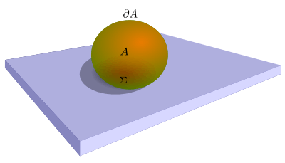
The content of this section and the following subsections follows closely the treatment of Gaetano Fichera in Fichera 1963, Fichera 1964b and also Fichera 1995: his derivation of the problem is different from Signorini's one in that he does not consider only incompressible bodies and a plane rest surface, as Signorini does.^[6] The problem consist in finding the displacement vector from the natural configuration $\scriptstyle\boldsymbol{u}(\boldsymbol{x})=\left(u_1(\boldsymbol{x}),u_2(\boldsymbol{x}),u_3(\boldsymbol{x})\right)$ of an anisotropic non-homogeneous elastic body that lies in a subset $A$ of the three-dimensional euclidean space whose boundary is $\scriptstyle\partial A$ and whose interior normal is the vector $n$ , resting on a rigid frictionless surface whose contact surface (or more generally contact set) is $\Sigma$ and subject only to its body forces $\scriptstyle\boldsymbol{f}(\boldsymbol{x})=\left(f_1(\boldsymbol{x}),f_2(\boldsymbol{x}),f_3(\boldsymbol{x})\right)$ , and surface forces $\scriptstyle\boldsymbol{g}(\boldsymbol{x})=\left(g_1(\boldsymbol{x}),g_2(\boldsymbol{x}),g_3(\boldsymbol{x})\right)$ applied on the free (i.e. 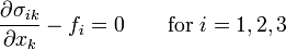not in contact with the rest surface) surface $\scriptstyle\partial A\setminus\Sigma$ : the set $A$ and the contact surface $\Sigma$ characterize the natural configuration of the body and are known a priori. Therefore the body has to satisfy the general equilibrium equations

(1)

\qquad\frac{\partial\sigma_{ik}}{\partial x_k}- f_i= 0\qquad\text{for } i=1,2,3

written using the Einstein notation as all in the following development, the ordinary boundary conditions on $\scriptstyle\partial A\setminus\Sigma$

(2)

\qquad\sigma_{ik}n_k-g_i=0\qquad\text{for } i=1,2,3

and the following two sets of boundary conditions on $\Sigma$ , where $\scriptstyle\boldsymbol{\sigma} = \boldsymbol{\sigma}(\boldsymbol{u})$ is the Cauchy stress tensor. Obviously, the body forces and surface forces cannot be given in arbitrary way but they must satisfy a condition in order for the body to reach an equilibrium configuration: this condition will be deduced and analized in the following development.

The ambiguous boundary conditions

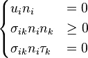
If $\scriptstyle\boldsymbol{\tau}=(\tau_1,\tau_2,\tau_3)$ is any tangent vector to the contact set $\Sigma$ , then the ambiguous boundary condition in each point of this set are expressed by the following two systems of inequalities

(3)

\quad \begin{cases} u_i n_i & = 0 \\ \sigma_{ik} n_i n_k & \geq 0\\ \sigma_{ik} n_i \tau_k & = 0 \end{cases}

or (4)

\begin{cases} u_i n_i & > 0 \\ \sigma_{ik} n_i n_k & = 0 \\ \sigma_{ik} n_i \tau_k & = 0 \end{cases}

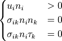
Let's analyze their meaning:

Each set of conditions consists of three relations, equalities or inequalities, and all the second members are the zero function.
The quantities at first member of each first relation are proportional to the norm of the component of the displacement vector directed along the normal vector $n$ .
The quantities at first member of each second relation are proportional to the norm of the component of the tension vector directed along the normal vector $n$ ,
The quantities at the first member of each third relation are proportional to the norm of the component of the tension vector along any vector $\tau$ tangent in the given point to the contact set $\Sigma$ .
The quantities at the first member of each of the three relations are positive if they have the same sense of the vector they are proportional to, while they are negative if not, therefore the constants of proportionality are respectively $\scriptstyle +1$ and $\scriptstyle -1$ .

Knowing these facts, the set of conditions (3) applies to points of the boundary of the body which do not leave the contact set $\Sigma$ in the equilibrium configuration, since, according to the first relation, the displacement vector $u$ has no components directed as the normal vector $n$ , while, according to the second relation, the tension vector may have a component directed as the normal vector $n$ and having the same sense. In an analogous way, the set of conditions (4) applies to points of the boundary of the body which leave that set in the equilibrium configuration, since displacement vector $u$ has a component directed as the normal vector $n$ , while the tension vector has no components directed as the normal vector $n$ . For both sets of conditions, the tension vector has no tangent component to the contact set, according to the hypothesis that the body rests on a rigid frictionless surface.

Each system expresses a unilateral constraint, in the sense that they express the physical impossibility of the elastic body to penetrate into the surface where it rests: the ambiguity is not only in the unknown values non-zero quantities must satisfy on the contact set but also in the fact that it is not a priori known if a point belonging to that set satisfies the system of boundary conditions (3) or (4). The set of points where (3) is satisfied is called the area of support of the elastic body on $\Sigma$ , while its complement respect to $\Sigma$ is called the area of separation.

The above formulation is general since the Cauchy stress tensor i.e. the constitutive equation of the elastic body has not been made explicit: it is equally valid assuming the hypothesis of linear elasticity or the ones of nonlinear elasticity. However, as it would be clear from the following developments, the problem is inherently nonlinear, therefore assuming a linear stress tensor does not simplify the problem.

The form of the stress tensor in the formulation of Signorini and Fichera

The form assumed by Signorini and Fichera for the elastic potential energy is the following one (as in the previous developments, the Einstein notation is adopted)

W(\boldsymbol{\varepsilon})=a_{ikjh}(\boldsymbol{x})\varepsilon_{ik}\varepsilon_{ik}

where

$\scriptstyle\boldsymbol{a}(\boldsymbol{x})=\left(a_{ikjh}(\boldsymbol{x})\right)$ is the elasticity tensor
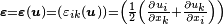$\scriptstyle\boldsymbol{\varepsilon}=\boldsymbol{\varepsilon}(\boldsymbol{u})=\left(\varepsilon_{ik}(\boldsymbol{u})\right)=\left(\frac{1}{2} \left( \frac{\partial u_i}{\partial x_k} + \frac{\partial u_k}{\partial x_i} \right)\right)$ is the infinitesimal strain tensor

The Cauchy stress tensor has therefore the following form

(5)

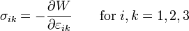
\sigma_{ik}= - \frac{\partial W}{\partial \varepsilon_{ik}} \qquad\text{for } i,k=1,2,3

and it is linear with respect to the components of the infinitesimal strain tensor; however, it is not homogeneous nor isotropic.

Solution of the problem

As for the section on the formal statement of the Signorini problem, the contents of this section and the included subsections follow closely the treatment of Gaetano Fichera in Fichera 1963, Fichera 1964b, Fichera 1972 and also Fichera 1995: obviously, the exposition focuses on the basics steps of the proof of the existence and uniqueness for the solution of problem (1), (2), (3), (4) and (5), rather than the technical details.

The potential energy

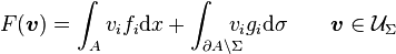
The first step of the analysis of Fichera as well as the first step of the analysis of Antonio Signorini in Signorini 1959 is the analysis of the potential energy, i.e. the following functional

(6)

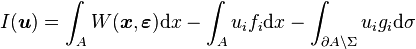
I(\boldsymbol{u})=\int_A W(\boldsymbol{x},\boldsymbol{\varepsilon})\mathrm{d}x - \int_A u_i f_i\mathrm{d}x - \int_{\partial A\setminus\Sigma}u_i g_i \mathrm{d}\sigma

where $u$ belongs to the set of admissible displacements $\scriptstyle\mathcal{U}_\Sigma$ i.e. the set of displacement vectors satisfying the system of boundary conditions (3) or (4). The meaning of each of the three terms is the following

the first one is the total elastic potential energy of the elastic body
the second one is the total potential energy due to the body forces, for example the gravitational force
the third one is the potential energy due to surface forces, for example the forces exerted by the atmospheric pressure

Signorini (1959, pp. 129–133) was able to prove that the admissible displacement $u$ which minimize the integral $I(u)$ is a solution of the problem with ambiguous boundary conditions (1), (2), (3), (4) and (5), provided it is a $C^1$ supported on the closure $\scriptstyle \bar A$ of the set $A$ : however Gaetano Fichera gave a class of counterexamples in (Fichera 1964b, pp. 619–620) showing that in general, admissible displacements are not smooth functions of these class. Therefore Fichera tries to minimize the functional (6) in a wider function space: in doing so, he first calculates the first variation (or functional derivative) of the given functional in the neighbourhood of the sought minimizing admissible displacement $\scriptstyle\boldsymbol{u} \in \mathcal{U}_\Sigma$ , and then requires it to be greater than or equal to zero

\left. \frac{\mathrm{d}}{\mathrm{d}t} I( \boldsymbol{u} + t \boldsymbol{v}) \right\vert_{t=0} = -\int_A \sigma_{ik}(\boldsymbol{u})\varepsilon_{ik}(\boldsymbol{v})\mathrm{d}x - \int_A v_i f_i\mathrm{d}x - \int_{\partial A\setminus\Sigma}\!\!\!\!\! v_i g_i \mathrm{d}\sigma \geq 0 \qquad \forall \boldsymbol{v} \in \mathcal{U}_\Sigma

Defining the following functionals

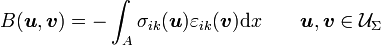
B(\boldsymbol{u},\boldsymbol{v}) = -\int_A \sigma_{ik}(\boldsymbol{u})\varepsilon_{ik}(\boldsymbol{v})\mathrm{d}x \qquad \boldsymbol{u},\boldsymbol{v} \in \mathcal{U}_\Sigma

and

F(\boldsymbol{v}) = \int_A v_i f_i\mathrm{d}x + \int_{\partial A\setminus\Sigma}\!\!\!\!\! v_i g_i \mathrm{d}\sigma\qquad \boldsymbol{v} \in \mathcal{U}_\Sigma

the preceding inequality is can be written as

(7)

B(\boldsymbol{u},\boldsymbol{v}) - F(\boldsymbol{v}) \geq 0 \qquad \forall \boldsymbol{v} \in \mathcal{U}_\Sigma

This inequality is the variational inequality for the Signorini problem.

Notes

↑ The exact Italian phrase is:- "Problema con ambigue condizioni al contorno".
↑ As Antonio Signorini himself writes in Signorini 1959, p. 129.
↑ See Fichera 1995, p. 49.
↑ This dramatic situation is well described by Fichera (1995, p. 51) himself.
↑ Fichera (1995, p. 53) reports the episode following the report of Mauro Picone: see the entry "Antonio Signorini" for further details.
↑ See Signorini 1959, p. 127) for the original approach.

Historical references

Antman, Stuart (1983), "The influence of elasticity in analysis: modern developments", Bulletin of the American Mathematical Society 9 (3): 267–291, doi:10.1090/S0273-0979-1983-15185-6, MR 714990, Zbl 0533.73001 .
Fichera, Gaetano (1972), "Boundary value problems of elasticity with unilateral constraints", in Flügge, Siegfried; Truesdell, Clifford A., Festkörpermechanik/Mechanics of Solids, Handbuch der Physik (Encyclopedia of Physics), VIa/2 (paperback 1984 ed.), Berlin–Heidelberg–New York: Springer-Verlag, pp. 391–424, ISBN 0-387-13161-2, Zbl 0277.73001 . The encyclopedia entry about problems with unilateral constraints (the class of boundary value problems the Signorini problem belongs to) he wrote for the Handbuch der Physik on invitation by Clifford Truesdell.
Fichera, Gaetano (1995), "La nascita della teoria delle disequazioni variazionali ricordata dopo trent'anni", Incontro scientifico italo-spagnolo. Roma, 21 ottobre 1993, Atti dei Convegni Lincei (in Italian) 114, Roma: Accademia Nazionale dei Lincei, pp. 47–53 . The birth of the theory of variational inequalities remembered thirty years later (English translation of the title) is an historical paper describing the beginning of the theory of variational inequalities from the point of view of its founder.
Fichera, Gaetano (2002), Opere storiche biografiche, divulgative (in Italian), Napoli: Giannini, p. 491 . "Historical, biographical, divulgative works" in the English translation: a volume collecting almost all works of Gaetano Fichera in the fields of history of mathematics and scientific divulgation.
Fichera, Gaetano (2004), Opere scelte, Firenze: Edizioni Cremonese (distributed by Unione Matematica Italiana), pp. XXIX+432 (vol. 1), pp. VI+570 (vol. 2), pp. VI+583 (vol. 3) , ISBN 88-7083-811-0 (vol. 1), ISBN 88-7083-812-9 (vol. 2), ISBN 88-7083-813-7 (vol. 3). Gaetano Fichera's "Selected works": three volumes collecting his most important mathematical papers, with a biographical sketch of Olga A. Oleinik.
Signorini, Antonio (1991), Opere scelte, Firenze: Edizioni Cremonese (distributed by Unione Matematica Italiana), pp. XXXI + 695 . The "Selected works" of Antonio Signorini: a volume collecting his most important works with an introduction and a commentary of Giuseppe Grioli.

References

Fichera, Gaetano (1963), "Sul problema elastostatico di Signorini con ambigue condizioni al contorno", Rendiconti della Accademia Nazionale dei Lincei, Classe di Scienze Fisiche, Matematiche e Naturali, 8 (in Italian) 34 (2): 138–142, Zbl 0128.18305 . "On the elastostatic problem of Signorini with ambiguous boundary conditions" (English translation of the title) is a short research note announcing and describing the solution of the Signorini problem.
Fichera, Gaetano (1964a), "Problemi elastostatici con vincoli unilaterali: il problema di Signorini con ambigue condizioni al contorno", Memorie della Accademia Nazionale dei Lincei, Classe di Scienze Fisiche, Matematiche e Naturali, 8 (in Italian) 7 (2): 91–140, Zbl 0146.21204 . "Elastostatic problems with unilateral constraints: the Signorini problem with ambiguous boundary conditions" (English translation of the title) is the first paper where aa existence and uniqueness theorem for the Signorini problem is proved.
Fichera, Gaetano (1964b), "Elastostatic problems with unilateral constraints: the Signorini problem with ambiguous boundary conditions", Seminari dell'istituto Nazionale di Alta Matematica 1962–1963, Rome: Edizioni Cremonese, pp. 613–679 . An English translation of the previous paper.
Signorini, Antonio (1959), "Questioni di elasticità non linearizzata e semilinearizzata", Rendiconti di Matematica e delle sue applicazioni, 5 (in Italian) 18: 95–139, Zbl 0091.38006 . "Topics in non linear and semilinear elasticity" (English translation of the title).

External links

Barbu, V. (2001), "Signorini problem", in Hazewinkel, Michiel, Encyclopedia of Mathematics, Springer, ISBN 978-1-55608-010-4