Shanks transformation
In numerical analysis, the Shanks transformation is a non-linear series acceleration method to increase the rate of convergence of a sequence. This method is named after Daniel Shanks, who rediscovered this sequence transformation in 1955. It was first derived and published by R. Schmidt in 1941.[1]
One can calculate only a few terms of a perturbation expansion, usually no more than two or three, and almost never more than seven. The resulting series is often slowly convergent, or even divergent. Yet those few terms contain a remarkable amount of information, which the investigator should do his best to extract.
This viewpoint has been persuasively set forth in a delightful paper by Shanks (1955), who displays a number of amazing examples, including several from fluid mechanics.
Formulation
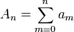
For a sequence  the series

is to be determined. First, the partial sum  is defined as:
and forms a new sequence  . Provided the series converges, will also approach the limit
  as
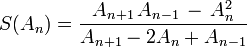
as  The Shanks transformation
  of the sequence is defined as[2][3]
and forms a new sequence. The sequence often converges more rapidly than the sequence  Further speed-up may be obtained by repeated use of the Shanks transformation, by computing
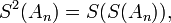
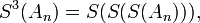 etc.
etc.
Note that the non-linear transformation as used in the Shanks transformation is essentially the same as used in Aitken's delta-squared process. Both operate on a sequence, but the sequence the Shanks transformation operates on is usually thought of as being a sequence of partial sums, although any sequence may be viewed as a sequence of partial sums.
Example
 in the partial sums and after applying the Shanks transformation once or several times:
 and
and  The series used is
 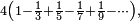 which has the exact sum
As an example, consider the slowly convergent series[3]
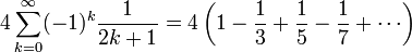
which has the exact sum π ≈ 3.14159265. The partial sum  has only one digit accuracy, while six-figure accuracy requires summing about 400,000 terms.
In the table below, the partial sums , the Shanks transformation on them, as well as the repeated Shanks transformations and  are given for up to 12. The figure to the right shows the absolute error for the partial sums and Shanks transformation results, clearly showing the improved accuracy and convergence rate.
| |
|
|
|
|
|---|---|---|---|---|
| 0 | 4.00000000 | — | — | — |
| 1 | 2.66666667 | 3.16666667 | — | — |
| 2 | 3.46666667 | 3.13333333 | 3.14210526 | — |
| 3 | 2.89523810 | 3.14523810 | 3.14145022 | 3.14159936 |
| 4 | 3.33968254 | 3.13968254 | 3.14164332 | 3.14159086 |
| 5 | 2.97604618 | 3.14271284 | 3.14157129 | 3.14159323 |
| 6 | 3.28373848 | 3.14088134 | 3.14160284 | 3.14159244 |
| 7 | 3.01707182 | 3.14207182 | 3.14158732 | 3.14159274 |
| 8 | 3.25236593 | 3.14125482 | 3.14159566 | 3.14159261 |
| 9 | 3.04183962 | 3.14183962 | 3.14159086 | 3.14159267 |
| 10 | 3.23231581 | 3.14140672 | 3.14159377 | 3.14159264 |
| 11 | 3.05840277 | 3.14173610 | 3.14159192 | 3.14159266 |
| 12 | 3.21840277 | 3.14147969 | 3.14159314 | 3.14159265 |
The Shanks transformation  already has two-digit accuracy, while the original partial sums only establish the same accuracy at
  Remarkably,
  has six digits accuracy, obtained from repeated Shank transformations applied to the first seven terms
  , ... ,
  As said before, only obtains 6-digit accuracy after about summing 400,000 terms.
Motivation
The Shanks transformation is motivated by the observation that — for larger — the partial sum quite often behaves approximately as[2]
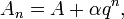
with  so that the sequence converges transiently to the series result for
So for
so that the sequence converges transiently to the series result for
So for  and
and  the respective partial sums are:

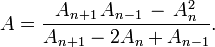
These three equations contain three unknowns: 
 and
and  Solving for gives[2]
In the (exceptional) case that the denominator is equal to zero: then  for all
Generalized Shanks transformation
The generalized kth-order Shanks transformation is given as the ratio of the determinants:[4]
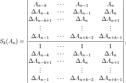
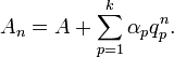
with 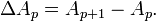 It is the solution of a model for the convergence behaviour of the partial sums with
  distinct transients:
This model for the convergence behaviour contains  unknowns. By evaluating the above equation at the elements
  and solving for the above expression for the kth-order Shanks transformation is obtained. The first-order generalized Shanks transformation is equal to the ordinary Shanks transformation:
The generalized Shanks transformation is closely related to Padé approximants and Padé tables.[4]
See also
Notes
References
- Shanks, D. (1955), "Non-linear transformation of divergent and slowly convergent sequences", Journal of Mathematics and Physics 34: 1–42
- Schmidt, R. (1941), "On the numerical solution of linear simultaneous equations by an iterative method", Philosophical Magazine 32: 369–383
- Van Dyke, M.D. (1975), Perturbation methods in fluid mechanics (annotated ed.), Parabolic Press, ISBN 0-915760-01-0
- Bender, C.M.; Orszag, S.A. (1999), Advanced mathematical methods for scientists and engineers, Springer, ISBN 0-387-98931-5
- Weniger, E.J. (2003). "Nonlinear sequence transformations for the acceleration of convergence and the summation of divergent series". v1. arXiv:math.NA/0306302.