Sequential minimal optimization
| Class | Optimization algorithm for training support vector machines |
|---|---|
| Worst case performance | O(n³) |
Sequential minimal optimization (SMO) is an algorithm for solving the quadratic programming (QP) problem that arises during the training of support vector machines. It was invented by John Platt in 1998 at Microsoft Research.[1] SMO is widely used for training support vector machines and is implemented by the popular LIBSVM tool.[2][3] The publication of the SMO algorithm in 1998 has generated a lot of excitement in the SVM community, as previously available methods for SVM training were much more complex and required expensive third-party QP solvers.[4]
Optimization problem
Consider a binary classification problem with a dataset (x1, y1), ..., (xn, yn), where xi is an input vector and yi ∈ {-1, +1} is a binary label corresponding to it. A soft-margin support vector machine is trained by solving a quadratic programming problem, which is expressed in the dual form as follows:
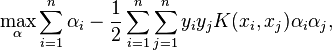
- subject to:


where C is an SVM hyperparameter and K(xi, xj) is the kernel function, both supplied by the user; and the variables  are Lagrange multipliers.
Algorithm
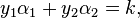
SMO is an iterative algorithm for solving the optimization problem described above. SMO breaks this problem into a series of smallest possible sub-problems, which are then solved analytically. Because of the linear equality constraint involving the Lagrange multipliers , the smallest possible problem involves two such multipliers. Then, for any two multipliers  and
and  , the constraints are reduced to:

and this reduced problem can be solved analytically: one needs to find a minimum of a one-dimensional quadratic function.  is the negative of the sum over the rest of terms in the equality constraint, which is fixed in each iteration.
The algorithm proceeds as follows:
- Find a Lagrange multiplier that violates the Karush–Kuhn–Tucker (KKT) conditions for the optimization problem.
- Pick a second multiplier and optimize the pair
 .
. - Repeat steps 1 and 2 until convergence.
When all the Lagrange multipliers satisfy the KKT conditions (within a user-defined tolerance), the problem has been solved. Although this algorithm is guaranteed to converge, heuristics are used to choose the pair of multipliers so as to accelerate the rate of convergence.
See also
References
- ↑ Platt, John (1998), Sequential Minimal Optimization: A Fast Algorithm for Training Support Vector Machines, CiteSeerX: 10
.1 .1 .43 .4376 - ↑ Chang, Chih-Chung; Lin, Chih-Jen (2011). "LIBSVM: A library for support vector machines". ACM Transactions on Intelligent Systems and Technology 2 (3).
- ↑ Luca Zanni (2006). Parallel Software for Training Large Scale Support Vector Machines on Multiprocessor Systems.
- ↑ Rifkin, Ryan (2002), "Everything Old is New Again: a Fresh Look at Historical Approaches in Machine Learning", Ph.D. thesis: 18