Semilinear response

The driving induces transitions between levels of a closed system, leading to diffusion in energy space and, hence, an associated heating. The diffusion coefficient can be calculated using a resistor network analogy.

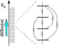
Semi-linear response theory (SLRT) is an extension of linear response theory (LRT) for mesoscopic circumstances: LRT applies if the driven transitions are much weaker/slower than the environmental relaxation/dephasing effect, while SLRT assumes the opposite conditions. SLRT uses a resistor network analogy (see illustration) in order to calculate the rate of energy absorption: The driving induces transitions between energy levels, and connected sequences of transitions are essential in order to have a non-vanishing result, as in the theory of percolation.

Applications

The original motivation for introducing SLRT was the study of mesosopic conductance ^[1] ^[2] ^[3] .^[4] The term SLRT has been coined in ^[5] where it has been applied to the calculation of energy absorption by metallic grains. Later the theory has been applied for analysing the rate of heating of atoms in vibrating traps .^[6]

Definition of semilinear response

Consider a system that is driven by a source $f(t)$ that has a power spectrum $\tilde{S}(\omega)$ . The latter is defined as the Fourier transform of $\langle f(t)f(0)\rangle$ . In linear response theory (LRT) the driving source induces a steady state which is only slightly different from the equilibrium state. In such circumstances the response ( $G$ ) is a linear functional of the power spectrum:

G = G[\tilde{S}(\omega)] = \int_{-\infty}^\infty \eta(\omega) \tilde{S}(\omega) \, d\omega

In the traditional LRT context $G$ represents the rate of heating, and $\eta(\omega)$ can be defined as the absorption coefficient. Whenever such relation applies

[A] \ \ \ \ \tilde{S}(\omega) \mapsto \lambda \tilde{S}(\omega) \text{ implies } G \mapsto \lambda G

[B] \ \ \ \ \tilde{S}(\omega) \mapsto \tilde{S}_1(\omega) + \tilde{S}_2(\omega) \text{ implies } G \mapsto G_1 + G_2

If the driving is very strong the response becomes non-linear, meaning that both properties [A] and [B] do not hold. But there is a class of systems whose response becomes semi-linear, i.e. the first property [A] still holds, but not [B].

Resistor network modeling

SLRT applies whenever the driving is strong enough such that relaxation to the steady state is slow compared with the driven dynamics. Yet one assumes that the system can be modeled as a resistor network, mathematically expressed as $G=[[G_{nm}]]$ . The notation $[[G_{nm}]]$ stands for the usual electrical engineering calculation of a two terminal conductance of a given resistor network. For example parallel connections imply $G = \sum_{nm} G_{nm}$ , while serial connections imply $G=\left[\sum_{nm} G_{nm}^{-1}\right]^{-1}$ . Resistor network calculation is manifestly semi-linear because it satisfies $[[\lambda A]]=\lambda [[A]]$ , but in general $[[A+B]]\ne[[A]]+[[B]]$ .

Fermi golden rule picture

In the quantum mechanical calculation of energy absorption, the $G_{nm}$ represent Fermi-golden-rule transition rates between energy levels. If only neighboring levels are coupled, serial addition implies

G = G[\tilde{S}(\omega)] = \left[\int_{-\infty}^\infty \mu(\omega) \tilde{S}(\omega)^{-1} \, d\omega\right]^{-1}

which is manifestly semi-linear. Results for sparse networks, that are encountered in the analysis of weakly chaotic driven systems, are more interesting and can be obtained using a generalized variable range hopping (VRH) scheme.

References

↑ D. Cohen, T. Kottos, H. Schanz, J. Phys. A 39, 11755 (2006)
↑ S. Bandopadhyay, Y. Etzioni and D. Cohen, Europhys. Lett. 76, 739 (2006)
↑ A. Stotland, R. Budoyo, T. Peer, T. Kottos, D. Cohen, J. Phys. A 41, 262001(FTC) (2008)
↑ A. Stotland, T. Kottos, D. Cohen, Phys. Rev. B 81, 115464 (2010)
↑ M. Wilkinson, B. Mehlig, D. Cohen, Europhys. Lett. 75, 709 (2006)
↑ A. Stotland, D. Cohen, N. Davidson, Europhys. Lett. 86, 10004 (2009)