Schur complement
In linear algebra and the theory of matrices, the Schur complement of a matrix block (i.e., a submatrix within a larger matrix) is defined as follows. Suppose A, B, C, D are respectively p×p, p×q, q×p and q×q matrices, and D is invertible. Let
![M=\left[\begin{matrix} A & B \\ C & D \end{matrix}\right]](../I/m/66eb0aebf60bfc9e21dabb25f1e399fe.png)
so that M is a (p+q)×(p+q) matrix.
Then the Schur complement of the block D of the matrix M is the p×p matrix

It is named after Issai Schur who used it to prove Schur's lemma, although it had been used previously.[1] Emilie Haynsworth was the first to call it the Schur complement.[2] The Schur complement is a key tool in the fields of numerical analysis, statistics and matrix analysis.
Background
The Schur complement arises as the result of performing a block Gaussian elimination by multiplying the matrix M from the right with the "block lower triangular" matrix
![L=\left[\begin{matrix} I_p & 0 \\ -D^{-1}C & I_q \end{matrix}\right].](../I/m/c7f5769da89379638d765ec3258a8ccd.png)
Here Ip denotes a p×p identity matrix. After multiplication with the matrix L the Schur complement appears in the upper p×p block. The product matrix is
![\begin{align}
ML &= \left[\begin{matrix} A & B \\ C & D \end{matrix}\right]\left[\begin{matrix} I_p & 0 \\ -D^{-1}C & I_q \end{matrix}\right] = \left[\begin{matrix} A-BD^{-1}C & B \\ 0 & D \end{matrix}\right] \\
&= \left[\begin{matrix} I_p & BD^{-1} \\ 0 & I_q \end{matrix}\right] \left[\begin{matrix} A-BD^{-1}C & 0 \\ 0 & D \end{matrix}\right].
\end{align}](../I/m/030cadfbde90d399cc087e467d41f677.png)
This is analogous to an LDU decomposition. That is, we have shown that
![\begin{align}
\left[\begin{matrix} A & B \\ C & D \end{matrix}\right] &= \left[\begin{matrix} I_p & BD^{-1} \\ 0 & I_q \end{matrix}\right] \left[\begin{matrix} A-BD^{-1}C & 0 \\ 0 & D \end{matrix}\right]
\left[ \begin{matrix} I_p & 0 \\ D^{-1}C & I_q \end{matrix}\right],
\end{align}](../I/m/6bdeb4aa8ade3e6a8a289cdba13d41db.png)
and inverse of M thus may be expressed involving D−1 and the inverse of Schur's complement (if it exists) only as
![\begin{align}
& {} \quad \left[ \begin{matrix} A & B \\ C & D \end{matrix}\right]^{-1} =
\left[ \begin{matrix} I_p & 0 \\ -D^{-1}C & I_q \end{matrix}\right]
\left[ \begin{matrix} (A-BD^{-1}C)^{-1} & 0 \\ 0 & D^{-1} \end{matrix}\right]
\left[ \begin{matrix} I_p & -BD^{-1} \\ 0 & I_q \end{matrix}\right] \\[12pt]
& = \left[ \begin{matrix} \left(A-B D^{-1} C \right)^{-1} & -\left(A-B D^{-1} C \right)^{-1} B D^{-1} \\ -D^{-1}C\left(A-B D^{-1} C \right)^{-1} & D^{-1}+ D^{-1} C \left(A-B D^{-1} C \right)^{-1} B D^{-1} \end{matrix} \right].
\end{align}](../I/m/9adc66c61489612b9ebdda859b1e5731.png)
C.f. matrix inversion lemma which illustrates relationships between the above and the equivalent derivation with the roles of A and D interchanged.
If M is a positive-definite symmetric matrix, then so is the Schur complement of D in M.
If p and q are both 1 (i.e. A, B, C and D are all scalars), we get the familiar formula for the inverse of a 2-by-2 matrix:
![M^{-1} = \frac{1}{AD-BC} \left[ \begin{matrix} D & -B \\ -C & A \end{matrix}\right]](../I/m/10c05307fdc01f8faa6cfe961e13cad6.png)
provided that AD − BC is non-zero.
Moreover, the determinant of M is also clearly seen to be given by

which generalizes the determinant formula for 2x2 matrices.
Application to solving linear equations
The Schur complement arises naturally in solving a system of linear equations such as
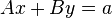

where x, a are p-dimensional column vectors, y, b are q-dimensional column vectors, and A, B, C, D are as above. Multiplying the bottom equation by  and then subtracting from the top equation one obtains

Thus if one can invert D as well as the Schur complement of D, one can solve for x, and
then by using the equation 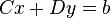 one can solve for y. This reduces the problem of
inverting a
one can solve for y. This reduces the problem of
inverting a  matrix to that of inverting a p×p matrix and a q×q matrix. In practice one needs D to be well-conditioned in order for this algorithm to be numerically accurate.
In electrical engineering this is often referred to as node elimination or Kron reduction.
Applications to probability theory and statistics
Suppose the random column vectors X, Y live in Rn and Rm respectively, and the vector (X, Y) in Rn+m has a multivariate normal distribution whose covariance is the symmetric positive-definite matrix
![\Sigma=\left[\begin{matrix} A & B \\ B^T & C \end{matrix}\right],](../I/m/2a92d3d63eb359a6491bde57a186a575.png)
where  is the covariance matrix of X,
  is the covariance matrix of Y and
  is the covariance matrix between X and Y.
Then the conditional covariance of X given Y is the Schur complement of C in  :
:


If we take the matrix above to be, not a covariance of a random vector, but a sample covariance, then it may have a Wishart distribution. In that case, the Schur complement of C in also has a Wishart distribution.
Schur complement condition for positive definiteness
Let X be a symmetric matrix given by
![X=\left[\begin{matrix} A & B \\ B^T & C \end{matrix}\right].](../I/m/206e6d8105b5e34b9985b14077c55d99.png)
Let S be the Schur complement of A in X, that is:

Then
-
 is positive definite if and only if
  and
and  are both positive definite:
 .
.
- is positive definite if and only if
 and
and  are both positive definite:
 .
.
- If is positive definite, then is positive semidefinite if and only if is positive semidefinite:

 ,
, 
 .
.
- If is positive definite, then is positive semidefinite if and only if is positive semidefinite:
-
 ,
,  .
.
The first and third statements can be derived[3] by considering the minimizer of the quantity
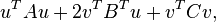
as a function of v (for fixed u).
Furthermore, since
![\left[\begin{matrix} A & B \\ B^T & C \end{matrix}\right] \succ 0 \Longleftrightarrow \left[\begin{matrix} C & B^T \\ B & A \end{matrix}\right] \succ 0](../I/m/7d704e830a1268298980dfbe1f324dcb.png)
and similarly for positive semi-definite matrices, the second (respectively fourth) statement is immediate from the first (resp. third).
See also
- Woodbury matrix identity
- Quasi-Newton method
- Haynsworth inertia additivity formula
- Gaussian process
- Total least squares
References
- ↑ Zhang, Fuzhen (2005). The Schur Complement and Its Applications. Springer. doi:10.1007/b105056. ISBN 0-387-24271-6.
- ↑ Haynsworth, E. V., "On the Schur Complement", Basel Mathematical Notes, #BNB 20, 17 pages, June 1968.
- ↑ Boyd, S. and Vandenberghe, L. (2004), "Convex Optimization", Cambridge University Press (Appendix A.5.5)