S transform
S transform as a time–frequency distribution was developed in 1994 for analyzing geophysics data.[1][2] In this way, the S transform is a generalization of the short-time Fourier transform (STFT), extending the continuous wavelet transform and overcoming some of its disadvantages. For one, modulation sinusoids are fixed with respect to the time axis; this localizes the scalable Gaussian window dilations and translations in S transform. Moreover, the S transform doesn't have a cross-term problem and yields a better signal clarity than Gabor transform. However, the S transform has its own disadvantages: it requires higher complexity computation (because FFT cannot be used), and the clarity is worse than Wigner distribution function and Cohen's class distribution function.
A fast S Transform algorithm was invented in 2010.[3] It reduces the computational time and resources by at least 4 orders of magnitude[4] and is available to the research community under an open source license.[5]
Definition
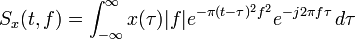
There are several ways to represent the idea of the S transform. In here, S transform is derived as the phase correction of the continuous wavelet transform with window being the Gaussian function.
- S-Transform
- Inverse S-Transform
![x(\tau) = \int_{-\infty}^{\infty}\left[\int_{-\infty}^{\infty}S_x(t,f)\, dt\right]\,e^{j2\pi f\tau}\, df](../I/m/9d522d6c70e523430ba066c7fc02e78c.png)
Modified Form
- Spectrum Form
The above definition implies that the s-transform function can be express as the convolution of 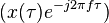 and
and  .
.
Applying the Fourier Transform to both and gives
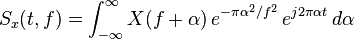 .
.
- Discrete Time S-transform
From the Spectrum Form of S-tansform, we can derive the discrete time S-transform.
Let  , where
  is the sampling interval and
  is the sampling frequency.
The Discrete time S-transform can then be expressed as:
![S_{x}(n\Delta_{T}\, ,m\Delta_{F}) = \sum_{p=0}^{N-1} X[(p+m)\,\Delta_{F}]\,e^{-\pi\frac{p^2}{m^2}}\,e^{\frac{j2pn}{N}}](../I/m/e9cb953ca5fb4c6c34de8bc015a63fb0.png)
Implementation of Discrete Time S-transform
Below is the Pseudo code of the implementation.
Step1.Compute![X[p\Delta_{F}]\,](../I/m/77cc6d023dd7e2c9a35c2761253a6e18.png)
loop{ Step2.Computefor
Step3.Moveto
Step4.Multiply Step2 and Step3
Step5.IDFT(). Repeat.}

![X[(p+m)\Delta_{F}]](../I/m/dd2720e408824e7345e75053ae69d14a.png)
![B[m,p] = X[(p+m)\Delta_{F}]\cdot e^{-\pi \frac{p^2}{m^2}}](../I/m/807db94b39fb98790bfaa1cc6089c63c.png)
Comparison with other Time-Frequency Analysis tools
- Compare with Gabor Transform
The only difference between Gabor Transform(GT) and S Transform is the window size. For GT, the windows size is a Gaussian function  , meanwhile, the window function for S-Transform is a function of f.
With a window function proportional to frequency, S Transform performs well in frequency domain analysis when the input frequency is low.When the input frequency is high, S-Transform have a better clarity in the time domain. As table below.
, meanwhile, the window function for S-Transform is a function of f.
With a window function proportional to frequency, S Transform performs well in frequency domain analysis when the input frequency is low.When the input frequency is high, S-Transform have a better clarity in the time domain. As table below.
| Low-frequency | Bad clarity in time domain | Good clarity in frequency domain |
| High-frequency | Bad clarity in frequency domain | Good clarity in time domain |
This kind of property makes S-Transform a powerful tool to analyze sound because human is sensitive to low frequency part in a sound signal.
- Compare with Wigner Transform
The main problem of Wigner Transform is the cross term which caused by the auto-correlation function in the Wigner Transform function. Cross term may cause noise and distortion to signal analysis. No cross term may appear by using the S-transform analysis which makes S Transform a suitable tool to design filter or signal modulation.
Discussion
We can compare the S transform and short-time Fourier transform (STFT).[2] First, a high frequency signal, a low frequency signal, and a high frequency burst signal are used in the experiment to compare the performance. The S transform characteristic of frequency dependent resolution allows the detection of the high frequency burst. On the other hand, as the STFT consists of a constant window width, it leads to the result having poorer definition. In the second experiment, two more high frequency bursts are added to crossed chirps. In the result, all four frequencies were detected by the S transform. On the other hand, the two high frequencies bursts are not detected by STFT. The high frequencies bursts cross term caused STFT to have a single frequency at lower frequency.
Applications
- Signal filterings[6]
- Magnetic resonance imaging (MRI)[7]
- Power system disturbance recognition
- S transform has been proven to be able to identify a few types of disturbances, like voltage sag, voltage swell, momentary interruption, and oscillatory transients.
- S transform also be applied for other types of disturbances such as notches, harmonics with sag and swells etc.
- S transform generates contours which are suitable for simple visual inspection. However, wavelet transform requires specific tools like standard multiresolution analysis.
- Geophysical signal analysis
See also
References
- ↑ Stockwell, RG, L Mansinha, and RP Lowe (1996). Localization of the complex spectrum: the S transform, IEEE Transactions on Signal Processing 44 (4), p 998-1001.
- ↑ 2.0 2.1 Stockwell, RG (1999). S-transform analysis of gravity wave activity from a small scale network of airglow imagers. PhD thesis, University of Western Ontario, London, Ontario, Canada.
- ↑ R. A. Brown and R. Frayne, "A fast discrete S-transform for biomedical signal processing", University of Calgary Seaman Family MR Research Centre Foothills Medical Centre, Canada. http://www.ncbi.nlm.nih.gov/pubmed/19163232
- ↑ Kelly Sansom, "Fast S Transform", University of Calgary, http://www.ucalgary.ca/news/utoday/may31-2011/computing
- ↑ http://sourceforge.net/projects/fst-uofc/
- ↑ Ditommaso, R, Mucciarelli M, Ponzo FC (2012). ANALYSIS OF NONSTATIONARY STRUCTURAL SYSTEMS BY USING A BAND-VARIABLE FILTER. Bulletin of Earthquake Engineering. doi:10.1007/s10518-012-9338-y. See also MATLAB file
- ↑ Hongmei Zhu, and J. Ross Mitchell, "The S Transform in Medical Imaging," University of Calgary Seaman Family MR Research Centre Foothills Medical Centre, Canada.
- Rocco Ditommaso, Marco Mucciarelli, Felice C. Ponzo (2010). S-Transform based filter applied to the analysis of non-linear dynamic behaviour of soil and buildings. 14th European Conference on Earthquake Engineering. Proceedings Volume. Ohrid, Republic of Macedonia. August 30 – September 3, 2010. (downloadable from http://roccoditommaso.xoom.it)
- M. Mucciarelli, M. Bianca, R. Ditommaso, M.R. Gallipoli, A. Masi, C Milkereit, S. Parolai, M. Picozzi, M. Vona (2011). FAR FIELD DAMAGE ON RC BUILDINGS: THE CASE STUDY OF NAVELLI DURING THE L’AQUILA (ITALY) SEISMIC SEQUENCE, 2009. Bulletin of Earthquake Engineering. doi:10.1007/s10518-010-9201-y.
- J. J. Ding, "Time-frequency analysis and wavelet transform course note," the Department of Electrical Engineering, National Taiwan University (NTU), Taipei, Taiwan, 2007.
- Jaya Bharata Reddy, Dusmanta Kumar Mohanta, and B. M. Karan, "Power system disturbance recognition using wavelet and s-transform techniques," Birla institute of Technology, Mesra, Ranchi-835215, 2004.
- B. Boashash, "Notes on the use of the wigner distribution for time frequency signal analysis", IEEE Trans. on Acoust. Speech. and Signal Processing, vol. 26, no. 9, 1987
- R. N. Bracewell, The Fourier Transform and Its Applications, McGrawHill Book Company, New York, 1978
- E. O. Brigham, The Fast Fourier Transform, Prentice-Hall Inc., Englewood Cliffs, New Jersey, 1974
- L. Cohen (1989). Time-frequency distributions—A review, Proc. IEEE, 77 (7).
- I. Daubechies, "The wavelet transform, time-frequency localization and signal analysis", IEEE Trans. on Information Theory, vol. 36, no. 5, Sept. 1990
- M. Farge, "Wavelet transforms and their application to turbulence", Annual Review of Fluid Mechanics, vol. 24, pp. 395–457, 1992
- D. Gabor, "Theory of communication", J. Inst. Elect. Eng., vol. 93, no. 3, pp. 429–457, 1946
- P. Goupillaud, A. Grossmann, and J. Morlet, "Cycle-octave and related transforms in seismic analysis", Geoexploration, vol. 23 pp. 85–102, 1984
- F. Hlawatsch and G. F. Boudreuax-Bartels, "Linear and quadratic timefrequency signal representations", IEEE SP Magazine, pp. 21–67, April 1992
- O. Rioul and M. Vetterli, "Wavelets and signal processing", IEEE SP Magazine, vol. 8 pp. 14–38, 1991
- R. K. Young, Wavelet Theory and its Applications, Kluwer Academic Publishers, Dordrecht,1993