SURF
| Feature detection |
|---|
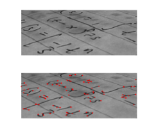 Output of a typical corner detection algorithm |
| Edge detection |
| Corner detection |
| Blob detection |
| Ridge detection |
| Hough transform |
| Structure tensor |
| Affine invariant feature detection |
| Feature description |
| Scale space |
In computer vision, SURF (Speeded Up Robust Features) is a robust local feature detector that can be used for tasks such as object recognition or 3D reconstruction. It is partly inspired by the SIFT descriptor. The standard version of SURF is several times faster than SIFT and claimed by its authors to be more robust against different image transformations than SIFT. SURF is based on sums of 2D Haar wavelet responses and makes an efficient use of integral images.
It uses an integer approximation of the determinant of Hessian blob detector, which can be computed extremely quickly with an integral image (with 3 integer operations). For features, it uses the sum of the Haar wavelet response around the point of interest. These can also be computed with the aid of the integral image. This information can be used to locate and recognize objects, people or faces, make 3D scenes, track objects and extract points of interest.
SURF was first presented by Herbert Bay et al. in 2006 at the European Conference on Computer Vision. An application of the algorithm is patented in the US.[1]
Overview
SURF is a detector and a high-performance descriptor for points of interest in images where the image is transformed into coordinates, using a technique called multi-resolution. Is to make a copy of the original image with Pyramidal Gaussian or Laplacian Pyramid shape and obtain image with the same size but with reduced bandwidth. Thus a special blurring effect on the original image, called Scale-Space is achieved. This technique ensures that the points of interest are scale invariant.
Algorithm and features
Detection
The SURF algorithm is based on the same principles and steps of SIFT, but it uses a different scheme and should provide better results faster. To detect scale-invariant characteristic points, the SIFT approach uses cascaded filters, where the difference of Gaussians (DoG), is calculated on rescaled images progressively.
Integral image
Instead of using Gaussian averaging, square-shaped filters are used as an approximation. Convolving the image with a square is much faster if the integral image is used. The integral image is defined as:
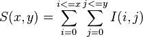
The sum of the original image within a rectangle D image can be evaluated quickly using the integral image. I(x, y) added over the selected area requires four evaluations S(x, y) (A, B, C, D)
Points of interest in the Hessian matrix
SURF uses a blob detector based on the Hessian to find points of interest. The determinant of the Hessian matrix expresses the extent of the response and is an expression of a local change around the area.
Blob structures are detected in places where the determinant of the Hessian is maximal. In contrast to the Hessian-Laplacian detector by Mikolajczyk and Schmid, SURF also uses the determinant of the Hessian for selecting the scale, as it is done by Lindeberg. Given a point p = (x, y) in an image I, the Hessian matrix H (p, σ) in p at scale σ, is defined as follows:
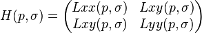
where  is the convolution of second order derivative
  with the image in the point x, y similarly with
  and
and  .
.
The Gaussian filters are optimal for scale space analysis, but in practice should be quantized and clipped. This leads to a loss of repeatability image rotations around the odd multiple of π / 4. This weakness is true for Hessian-based detectors in general. Repeatability of peaks around multiples of π / 2. This is due to the square shape of the filter. However, the detectors still work well, the discretization has a slight effect on performance. As real filters are not ideal, in any case, given the success of Lowe with logarithmic approximations, they push the approximation of the Hessian further matrix with square filters. These second order Gaussian filters' approximate can be evaluated with a cost very low with the use of integrated computer images. Therefore, the calculation time is independent of the filter size. Here are some approaches: Gyy and Gxy (1)
The box filters 9x9 are approximations of a Gaussian with σ = 1.2 and represents the lowest level ( higher spatial resolution ) for computerized maps BLOB response. Is denoted Dxx, Dyy, Dxy . The weights applied to the rectangular regions are maintained by the efficiency of the CPU.
Images are calculated :
-Dxx (x, y ) from I ( x, y) and Gxx ( x, y)
-Dxy (x, y ) from I ( x, y) and Gxy (x, y )
-Dyy (x, y ) from I ( x, y) and Gyy (x, y)
Then, the following image is generated:

The relative weighting (w) of the filter response is used to balance the expression for the Hessian determinant . It is necessary for the conservation of energy between Gaussian kernels and Gaussian kernels approximate.
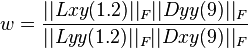
0.9 factor appears such a correction factor using squares instead of gaussians. it can generate several images det (H) for several filter sizes . This is called multi- resolution analysis.
 is the Frobenius norm: Frobenius
Changes of weighting depends on scale σ . In practice, this factor is kept constant . How it keep constant? Normalizing the filter response relative to its size. This ensures the Frobenius norm for any other filter.
The approximation of the determinant of the Hessian matrix representing the response BLOB image on location x . These responses are stored in the BLOB response map on different scales.
Then, the local maxima are searched.
Scale-space representation & location of points of interest
The attractions can be found in different scales, partly because the search for correspondences often requires comparison images where they are seen at different scales. The scale spaces are generally applied as a pyramid image . Images are repeatedly smoothed with a Gaussian filter, then, is sub sampled to achieve a higher level of the pyramid. Therefore, several floors or stairs " det H" with various measures of the masks are calculated:
The scale -space is divided into a number of octaves, Where an octave refers to a series of response maps of covering a doubling of scale . In SURF The Lowest level of the Scale- space is Obtained from the output of the 9 × 9 filters.
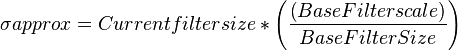
Scale spaces are implemented by applying box filters of different size. Therefore, the scale space is analyzed by up-scaling the filter size rather than iteratively reducing the image size. The output of the above 9*9 filter is considered as the initial scale layer, to which we will refer as scale s=1.2 (corresponding to Gaussian derivatives withσ=1.2). The following layers are obtained by filtering the image with gradually bigger masks, taking into account the discrete nature of integral images and the specific structure of or filters. Specifically, this results in filters of size 9*9, 15*15, 21*21, 27*27, etc. In order to localize interest points in the image and over scales, non-maximum suppression in a 3*3*3 neighborhood is applied. The maxima of the determinant of the Hessian matrix are then interpolated in scale and image space with the method proposed by Brown et al. Scale space interpolation is especially important in our case, as the difference in scale between the first layers of every octave is relatively large.
After 3D maxima are looking at ( x, y, n) using the cube 3x3x3 neighborhood . From there it is proceed to do the interpolation of the maximum. Lowe rest of the layers of the pyramid to get the DOG (Difference of Gaussian ) find images contours and stains.
Specifically, it is entered by variant a quick and Van Gool Neubecker used . The maximum of the determinant of the Hessian matrix in scale and space interpolated image with Brown and Lowe proposed method. The approach of the determinant of the Hessian matrix represents the response of BLOB in the image to the location x . These responses are stored in the BLOB map of responses on different scales. Them have the principal feature of repetibility, that means if some point is considerated realiable, the detector will find the same point under different perspective (scale, orientation, rotation, etc.).
It has one position (x,y) for each interest point.
Description
The goal of a descriptor is to provide a unique and robust description of an image feature, e.g. by describing the intensity distribution of the pixels within the neighborhood of the point of interest. Most descriptors are computed thus in a local manner; hence, a description is obtained for every point of interest identified previously.
The dimensionality of the descriptor has direct impact on both its computational complexity and point-matching robustness/accuracy. A short descriptor may be more robust against appearance variations, but may not offer sufficient discrimination and thus give too many false positives.
The next three introducing steps are explained in the following: The first step consists of fixing a reproducible orientation based on information from a circular region around the interest point. Then, we construct a square region aligned to the selected orientation and extract the SURF descriptor from it. Finally, features are matched between two images.
The SURF descriptor is based on the similar properties of SIFT, with a complexity stripped down even further. The first step consists of fixing a reproducible orientation based on information from a circular region around the interest point. The second step is constructing as square region aligned to the selected orientation, and extracting the SURF descriptor from it. These two steps are now explained in turn. Furthermore, we also propose an upright version of our descriptor (U-SURF) that is not invariant to image rotation and therefore faster to compute and better suited for application where the camera remains more or less horizontal.
Orientation Assignment
In order to achieve rotational invariance, the orientation of the point of interest needs to be found. The Haar wavelet responses in both x- and y-directions within a circular neighbourhood of radius  around the point of interest are computed, where
  is the scale at which the point of interest was detected. The obtained responses are weighed by a Gaussian function centered at the point of interest, then plotted as points in a two-dimensional space, with the horizontal response in the abscissa and the vertical response in the ordenate. The dominant orientation is estimated by calculating the sum of all responses within a sliding orientation window of size π/3. The horizontal and vertical responses within the window are summed. The two summed responses then yield a local orientation vector. The longest such vector overall defines the orientation of the point of interest. The size of the sliding window is a parameter which has to be chosen carefully to achieve a desired balance between robustness and angular resolution.
Descriptor based on Sum of Haar Wavelet Responses
For the extraction of the descriptor, the first step consist of constructing a square region centred around the interest 6point and oriented along the orientation selected in the previous section. The size of this window is 20s.
The interest region is split up into smaller 4x4 square sub-regions, and for each one, it is computed Haar wavelet responses at 5x5 regularly spaced sample points., and weighted with a Gaussian (to offer more robustness for deformations, noise and translations, This responses are dx and dy.
The select interest point orientation is who defines de horizontality and verticality.
For each sub-region the resultts of  ,
,  and their absolutes, are summed in a vector, the descriptor:

Which is distinctive and, at the same time, robust to noise, geometric and photometric distortions and errors. Surf descriptor obtained by the union of the sub- vectors .
Matching
This section details the step back in search of characteristic points that provides the detector. This way it is possible to compare between descriptors and look for matching pairs of images between them. There are two ways to do it:
- Get the characteristic points of the first image and its descriptor and do the same with the second image . So you will be able to compare the two images descriptor correspondences between points and establish some kind of measure.
- Get the characteristic points of the first image with the descriptor. Then compare this descriptor with the points of the second image which is believed to be the partner concerned.
Surf vs Sift
Presentation of the algorithms
The recognition of images or objects, is one of the most important applications of computer vision, becomes a comparison of local descriptors SIFT (Scale Invariant Feature Transform) [David Lowe, 1999] and SURF (Speeded-UP Feature transform) [Bay and Tuytelaars 2006]. These two local descriptors detect structures or very significant points in an image for a discriminating description of these areas from its neighboring points, in order to compare them with other descriptors using similar measures. Below are given some basic features of these two algorithms:
SIFT (Scale Invariant Feature Transform) was published by David Lowe in 1999 with the idea of proposing an algorithm capable of extracting the characteristics of an image already splitting of these describe the set of objects that were contained in it. This algorithm can be broken into 4 stages:
-Detection of edges on the scale: the first stage performs a search in different scales and dimensions of the image by identifying possible points of interest, invariant to changes in orientation and scaling. This procedure is carried out with the function (DoG (Difference-of-Gaussian) giving different values to the σ, in the following equation):

Where G is the Gaussian function and the I is the image. Now Gaussian images are subtracted in order to produce the DoG, after that is submostrea the Gaussian image by a factor of 2 to obtain a DoG image sampling. Each pixel is set with its neighbors with a mask 3 x 3 to find maxim and minim local of D (x, y, σ).
-Location of the keypoints: key points are chosen on the basis of stability measures, removed the key points with low.
-Contrast or are located in the margins-orientation assignment: invariance to rotation is achieved by assigning to each of the points of orientation based on the local properties of the image and which represents the descriptor for this orientation.
-Descriptor keypoints: the local gradients of the image are measured in the region surrounding the key point. These are processed by means of a representation which allows distortion levels and changes in lighting locally.
SURF (Speeded-UP Feature Transform) as we have seen in previous sections, the SURF is an algorithm developed by Herbert Bay, Tinne Tuytelaars and Luc Van Gool (2008), works as a detector and descriptor of sites focused on object recognition. This algorithm has 3 stages:
-Detection of points of interest, keypoints.
-Assignment guidance.
-Extraction of those described.More information in the sections of features.
Theoretical differences
The main differences between the algorithms SIFT and SURF are the speed of implementation of respect for one another, but with both points of interest of the image keep invariants, scale and orientation, and changes in the lighting. The main differences of data in multiple experiments are that SIFT is kept the position, scale and orientation, since it is possible that in a same position (x, and), we find several points of interest to different scale and / or orientation σ. But another side in the SURF in a position (x, and) appears only a single point of interest, by what is not saved the scale and orientation, however if that registers the matrix of second order and the sign of the Laplacian.
Experimental differences
Test 1
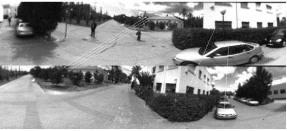
To make comparisons must take into account the versions of the algorithms that are used in each case, in this article obtained conclusions with version 4 of the Sift and SURF with C code version 1.0.9 and analyzing images with greyscale, are also drawn conclusions from results of experiments with robots and response of the algorithms in platforms Android. The result of tests with 109 images, as announced before, it has been confirmed that the SURF method is much faster than SIFT. From the point of view of invariant points detected, the SIFT algorithm outperforms surfing more than double points detected. This is caused because the SURF allows that multiple invariant points in a same position with different scale or orientation, while in the SIFT if that is possible there are. This fact means that the distance between the number of detected features would decrease if the SIFT not duplication of points. The graphs show that the SIFT method has some 2.68 invariant points that the SURF with respect to time, SIFT more used about 1646 ms to analyze an image and the SURF 485 ms, is almost one-third of the time, efficiency in this factor is considerable. This factor is important in face of the purpose of each project, if you want an algorithm that can get a great amount of data would be more advisable to SIFT, but a quick response is needed and we don't give so much importance to the number of detected features SURF algorithm is the most suitable.
| SIFT | SURF |
|---|---|
 |
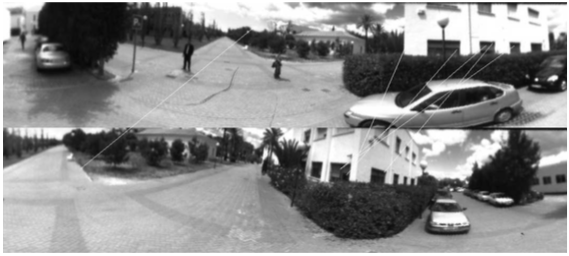 |
There is detail the order of the images by comparing the photo is very important, since results may vary if you choose a comparison with X vs and if done with and vs X. The SIFT method shows more points when the images being compared have more points in common, unlike the SURF gives more values when the images are more differentiated, false positive values. This happens with all photographs and leads to the conclusion that the SIFT algorithm has more durability in the time to SURF, obtaining more reliable pairings.
|
109 IMAGES |
SIFT | SURF |
|---|---|---|
| Detected points | 1292 | 482 |
| Average time | 1646.53 ms | 485.77 ms |
- Data extracted from an analysis made by A. M. Romero and M. Cazorla, in the document "comparison of detectors of Visual characteristics and its application to SLAM ”.
Test 2
The following study is an experiment of performance, consumption and efficiency of algorithms, in which 100 prepared logos have been and was executed 10 times each test in functionality, in order to see if the algorithms modify their behavior depending on the mobile device. The components of the testing scenario were the following:
Database: is a tuple consisting of a vector characteristics and other points of training Interes.
Training component: saves the database and points of interest generated by test algoritmos.
Try component: allows to get the vector of characteristics and interest points generated by each descriptor (SIFT, SURF) from a search (matching) input.
Search (matching): allows you to obtain a set of correspondences between the obtained tuple and tuple from the database.
| SIFT | SURF | |
|---|---|---|
| Average interest points | 222 | 431 |
| Runtime | 2887.13 ms | 959.87 ms |
| Power consumption | 0.04 % | 0.02 % |
| Memory used | 102.30 KB | 385.02 KB |
| Effectiveness | 0.33 | 0.40 |
In the previous table, the results obtained with regard to the points of interest is observed the difference from the average of points detected by the SIFT method much less than surfing, because of the difference in the compared images. Regarding runtime SIFT is much slower than the SURF, indicating that for real-time applications this algorithm should be ruled out. In battery consumption the results are proportional to the runtime, so SIFT consumes twice as much as the SURF method.Regarding the memory used SURF method exceeds the resources to store the vector of characteristics of images, almost four times more than the method SIFT on issues of effectiveness the SIFT method is also less effective than the SURF, but slightly lower.
See also
- Scale-invariant feature transform (SIFT)
- Gradient Location and Orientation Histogram
- LESH - Local Energy based Shape Histogram
- Blob detection
- Feature detection (computer vision)
References
- ↑ US 2009238460, Ryuji Funayama, Hiromichi Yanagihara, Luc Van Gool, Tinne Tuytelaars, Herbert Bay, "ROBUST INTEREST POINT DETECTOR AND DESCRIPTOR", published 2009-09-24
- Herbert Bay, Tinne Tuytelaars, and Luc Van Gool, "Speeded Up Robust Features", ETH Zurich, Katholieke Universiteit Leuven
- Andrea Maricela Plaza Cordero,Jorge Luis Zambrano Martínez, " Estudio y Selección de las Técnicas SIFT, SURF y ASIFT de Reconocimiento de Imágenes para el Diseño de un Prototipo en Dispositivos Móviles" , 15º Concurso de Trabajos Estudiantiles, EST 2012
- A. M. Romero and M. Cazorla, "Comparativa de detectores de característicasvisuales y su aplicación al SLAM ", X Workshop de agentes físicos, Setiembre 2009, Cáceres
- P. M. Panchal, S. R. Panchal, S. K. Shah, "A Comparison of SIFT and SURF ", International Journal of Innovative Research in Computer and Communication Engineering Vol. 1, Issue 2, April 2013
- Herbert Bay, Andreas Ess, Tinne Tuytelaars, Luc Van Gool "SURF: Speeded Up Robust Features", Computer Vision and Image Understanding (CVIU), Vol. 110, No. 3, pp. 346–359, 2008
- Christopher Evans "Notes on the OpenSURF Library", MSc Computer Science, University of Bristol