Root locus
In control theory and stability theory, root locus analysis is a graphical method for examining how the roots of a system change with variation of a certain system parameter, commonly a gain within a feedback system. This is a technique used as a stability criterion in the field of control systems developed by Walter R. Evans which can determine stability of the system. The root locus plots the poles of the closed loop transfer function as a function of a gain parameter.
Uses
In addition to determining the stability of the system, the root locus can be used to design the damping ratio and natural frequency of a feedback system. Lines of constant damping ratio can be drawn radially from the origin and lines of constant natural frequency can be drawn as arcs whose center points coincide with the origin. By selecting a point along the root locus that coincides with a desired damping ratio and natural frequency a gain, K, can be calculated and implemented in the controller. More elaborate techniques of controller design using the root locus are available in most control textbooks: for instance, lag, lead, PI, PD and PID controllers can be designed approximately with this technique.
The definition of the damping ratio and natural frequency presumes that the overall feedback system is well approximated by a second order system; i.e. the system has a dominant pair of poles. This is often not the case, so it is good practice to simulate the final design to check if the project goals are satisfied.
-(1_3_5_1).png)
Example
Suppose there is a feedback system whose input is the signal X(s) and output is Y(s). The feedback system forward path gain is G(s); the feedback path gain is H(s).

For this system, the overall transfer function is given by[1]
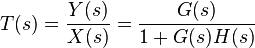
Thus the closed-loop poles (roots of the characteristic equation) of the transfer function are the solutions to the equation 1 + G(s)H(s) = 0. The principal feature of this equation is that roots may be found wherever G(s)H(s) = -1.
In systems without pure delay, the product G(s)H(s) = -1 is a rational polynomial function and may be expressed as[2]
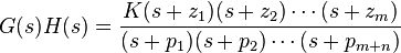
where the −zi are the m zeros, the −pi are the m + n poles, and K is a scalar gain. Typically, a root locus diagram will indicate the transfer function's pole locations for varying values of K. A root locus plot will be all those points in the s-plane where G(s)H(s) = -1 for any value of K.
The factoring of K and the use of simple monomials means the evaluation of the rational polynomial can be done with vector techniques that add or subtract angles and multiply or divide magnitudes. The vector formulation arises from the fact that each monomial term in the factored G(s)H(s), (s−a) for example, represents the vector from a to s. The polynomial can be evaluated by considering the magnitudes and angles of each of these vectors. According to vector mathematics, the angle of the result is the sum of all the angles in the numerator add minus the sum of all the angles in the denominator. Similarly, the magnitude of the result is the product of all the magnitudes in the numerator divided by the product of all the magnitudes in the denominator. It turns out that the calculation of the magnitude is not needed because K varies; one of its values may result in a root. So to test whether a point in the s-plane is on the root locus, only the angles to all the open loop poles and zeros need be considered. A graphical method that uses a special protractor called a "Spirule" was once used to determine angles and draw the root loci.[3]
From the function T(s), it can be seen that the value of K does not affect the location of the zeros. The root locus only gives the location of closed loop poles as the gain K is varied. The zeros of a system do not move.
Using a few basic rules, the root locus method can plot the overall shape of the path (locus) traversed by the roots as the value of K varies. The plot of the root locus then gives an idea of the stability and dynamics of this feedback system for different values of K.[4][5]
Sketching root locus
- Mark open-loop poles and zeros
- Mark real axis portion to the left of an odd number of poles and zeros
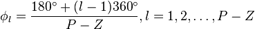
- Find asymptotes
Let P be the number of poles and Z be the number of zeros:

The asymptotes intersect the real axis at  (which is called the centroid) and depart at angle
  given by:
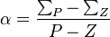
where  is the sum of all the locations of the poles, and
  is the sum of all the locations of the explicit zeros.
- Phase condition on test point to find angle of departure
- Compute breakaway/break-in points
The breakaway points are located at the roots of the following equation:
Once you solve for z, the real roots give you the breakaway/reentry points. Complex roots correspond to a lack of breakaway/reentry.
z-plane versus s-plane
The root locus method can also be used for the analysis of sampled data systems by computing the root locus in the z-plane, the discrete counterpart of the s-plane. The equation z = esT maps continuous s-plane poles (not zeros) into the z-domain, where T is the sampling period. The stable, left half s-plane maps into the interior of the unit circle of the z-plane, with the s-plane origin equating to |z| = 1 (because e0 = 1). A diagonal line of constant damping in the s-plane maps around a spiral from (1,0) in the z plane as it curves in toward the origin. Note also that the Nyquist aliasing criteria is expressed graphically in the z-plane by the x-axis, where ωnT = π. The line of constant damping just described spirals in indefinitely but in sampled data systems, frequency content is aliased down to lower frequencies by integral multiples of the Nyquist frequency. That is, the sampled response appears as a lower frequency and better damped as well since the root in the z-plane maps equally well to the first loop of a different, better damped spiral curve of constant damping. Many other interesting and relevant mapping properties can be described, not least that z-plane controllers, having the property that they may be directly implemented from the z-plane transfer function (zero/pole ratio of polynomials), can be imagined graphically on a z-plane plot of the open loop transfer function, and immediately analyzed utilizing root locus.
Since root locus is a graphical angle technique, root locus rules work the same in the z and s planes.
The idea of a root locus can be applied to many systems where a single parameter K is varied. For example, it is useful to sweep any system parameter for which the exact value is uncertain in order to determine its behavior.
See also
- Phase margin
- Routh–Hurwitz stability criterion
- Nyquist stability criterion
- Gain and phase margin
- Bode plot
References
- ↑ Kuo 1967, p. 331.
- ↑ Kuo 1967, p. 332.
- ↑ Evans, Walter R. (1965), Spirule Instructions, Whittier, CA: The Spirule Company
- ↑ Evans, W. R. (January 1948), "Graphical Analysis of Control Systems", Trans. AIEE 67 (1): 547–551, doi:10.1109/T-AIEE.1948.5059708, ISSN 0096-3860
- ↑ Evans, W. R. (January 1950), "Control Systems Synthesis by Root Locus Method", Trans. AIEE 69 (1): 66–69, doi:10.1109/T-AIEE.1950.5060121, ISSN 0096-3860
- Kuo, Benjamin C. (1967), "Root Locus Technique", Automatic Control Systems (second ed.), Englewood Cliffs, NJ: Prentice-Hall, pp. 329–388, ASIN B000KPT04C, LCCN 67016388, OCLC 3805225
Further reading
- Ash, R. H.; Ash, G. H. (October 1968), "Numerical Computation of Root Loci Using the Newton-Raphson Technique", IEEE Trans. Automatic Control 13 (5), doi:10.1109/TAC.1968.1098980
- Williamson, S. E. (May 1968), "Design Data to assist the Plotting of Root Loci (Part I)", Control Magazine 12 (119): 404–407
- Williamson, S. E. (June 1968), "Design Data to assist the Plotting of Root Loci (Part II)", Control Magazine 12 (120): 556–559
- Williamson, S. E. (July 1968), "Design Data to assist the Plotting of Root Loci (Part III)", Control Magazine 12 (121): 645–647
- Williamson, S. E. (May 15, 1969), "Computer Program to Obtain the Time Response of Sampled Data Systems", IEE Electronics Letters 5 (10): 209–210, doi:10.1049/el:19690159
- Williamson, S. E. (July 1969), "Accurate Root Locus Plotting Including the Effects of Pure Time Delay" (PDF), Proc. IEE 116 (7): 1269–1271, doi:10.1049/piee.1969.0235
External links
- Wikibooks: Control Systems/Root Locus
- Carnegie Mellon / University of Michigan Tutorial
- Excellent examples. Start with example 5 and proceed backwards through 4 to 1. Also visit the main page
- The root-locus method: Drawing by hand techniques
- "RootLocs": A free multi-featured root-locus plotter for Mac and Windows platforms
- "Root Locus": A free root-locus plotter/analyzer for Windows
- Root Locus at ControlTheoryPro.com
- Root Locus Analysis of Control Systems
- MATLAB function for computing root locus of a SISO open-loop model
- Wechsler, E. R. (January–March 1983), Root Locus Algorithms for Programmable Pocket Calculators (PDF), NASA, pp. 60–64, TDA Progress Report 42-73
- Mathematica function for plotting the root locus