Rogers–Ramanujan continued fraction
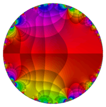
The Rogers–Ramanujan continued fraction is a continued fraction discovered by Rogers (1894) and independently by Srinivasa Ramanujan, and closely related to the Rogers–Ramanujan identities. It can be evaluated explicitly for a broad class of values of its argument.
 of the function
  , where
  is the Rogers–Ramanujan continued fraction.
Definition

 of the Rogers–Ramanujan continued fraction.
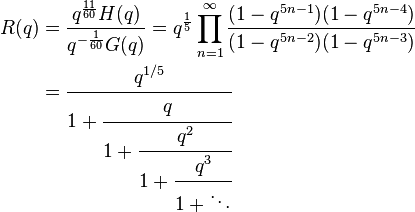
Given the functions G(q) and H(q) appearing in the Rogers–Ramanujan identities,
![\begin{align}G(q)
&= \sum_{n=0}^\infty \frac {q^{n^2}} {(q;q)_n} = \frac {1}{(q;q^5)_\infty (q^4; q^5)_\infty}\\
&= \prod_{n=1}^\infty \frac{1}{(1-q^{5n-1})(1-q^{5n-4})}\\
&=\sqrt[60]{qj}\,_2F_1\left(-\tfrac{1}{60},\tfrac{19}{60};\tfrac{4}{5};\tfrac{1728}{j}\right)\\
&=\sqrt[60]{q\left(j-1728\right)}\,_2F_1\left(-\tfrac{1}{60},\tfrac{29}{60};\tfrac{4}{5};-\tfrac{1728}{j-1728}\right)\\
&= 1+ q +q^2 +q^3 +2q^4+2q^5 +3q^6+\cdots
\end{align}](../I/m/98caf6d1e1d760b4027fa0e85e1369e2.png)
and,
![\begin{align}H(q)
&=\sum_{n=0}^\infty \frac {q^{n^2+n}} {(q;q)_n} = \frac {1}{(q^2;q^5)_\infty (q^3; q^5)_\infty}\\
&= \prod_{n=1}^\infty \frac{1}{(1-q^{5n-2})(1-q^{5n-3})}\\
&=\frac{1}{\sqrt[60]{q^{11}j^{11}}}\,_2F_1\left(\tfrac{11}{60},\tfrac{31}{60};\tfrac{6}{5};\tfrac{1728}{j}\right)\\
&=\frac{1}{\sqrt[60]{q^{11}\left(j-1728\right)^{11}}}\,_2F_1\left(\tfrac{11}{60},\tfrac{41}{60};\tfrac{6}{5};-\tfrac{1728}{j-1728}\right)\\
&= 1+q^2 +q^3 +q^4+q^5 +2q^6+2q^7+\cdots
\end{align}](../I/m/69a880daeb9ef696c628120b93da695f.png)
![]() A003114 and
A003114 and ![]() A003106, respectively, where
A003106, respectively, where  denotes the infinite q-Pochhammer symbol, j is the j-function, and 2F1 is the hypergeometric function, then the Rogers–Ramanujan continued fraction is,
Modular functions
If  , then
  and
and  , as well as their quotient , are modular functions of
  . Since they have integral coefficients, the theory of complex multiplication implies that their values for an imaginary quadratic irrational are algebraic numbers that can be evaluated explicitly.
Examples
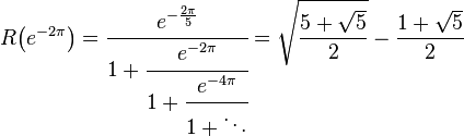

where 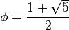 is the golden ratio.
Relation to modular forms
It can be related to the Dedekind eta function, a modular form of weight 1/2, as,[1]

![\frac{1}{R^5(q)}-R^5(q) = \left[\frac{\eta(\tau)}{\eta(5\tau)}\right]^6+11](../I/m/99b496525db7e04de0752095f35bfd9a.png)
Relation to j-function
Among the many formulas of the j-function, one is,

where,
![x = \left[\frac{\sqrt{5}\,\eta(5\tau)}{\eta(\tau)}\right]^6](../I/m/28391276099195314377c98e7056add2.png)
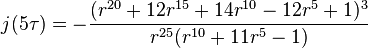
Eliminating the eta quotient, one can then express j(τ) in terms of  as,
as,


where the numerator and denominator are polynomial invariants of the icosahedron. Using the modular equation between and  , one finds that,
let ,then
,then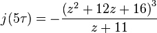
where,
![z_{\infty}= -\left[\frac{\sqrt{5}\,\eta(25\tau)}{\eta(5\tau)}\right]^6-11,z_0=-\left[\frac{\eta(\tau)}{\eta(5\tau)}\right]^6-11,z_1=\left[\frac{\eta(\frac{5\tau+2}{5})}{\eta(5\tau)}\right]^6-11,z_2=-\left[\frac{\eta(\frac{5\tau+4}{5})}{\eta(5\tau)}\right]^6-11,z_3=\left[\frac{\eta(\frac{5\tau+6}{5})}{\eta(5\tau)}\right]^6-11,z_4=-\left[\frac{\eta(\frac{5\tau+8}{5})}{\eta(5\tau)}\right]^6-11](../I/m/cb126db2bdd03afa47d4a6848b79bc23.png)
which in fact is the j-invariant of the elliptic curve,

parameterized by the non-cusp points of the modular curve  .
.
Functional equation
For convenience, one can also use the notation  when q = e2πiτ. While other modular functions like the j-invariant satisfies,
and the Dedekind eta function has,

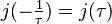
the functional equation of the Rogers–Ramanujan continued fraction involves[2] the golden ratio  ,
,
Incidentally,

Modular equations
There are modular equations between and  . Elegant ones for small prime n are as follows.[3]
For  , let
, let  and
and  , then
For  , let and
  , then
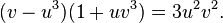
For  , let and
  , then
For  , let and
  , then
Regarding , note that 
Other results
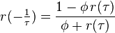
Ramanujan found many other interesting results regarding R(q).[4] Let  ,
,  , and as the golden ratio.
If  , then
If  , then
The powers of R(q) also can be expressed in unusual ways. For its cube,

For its fifth power, let 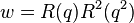 , then,

References
- ↑ Duke, W. "Continued Fractions and Modular Functions", http://www.math.ucla.edu/~wdduke/preprints/bams4.pdf
- ↑ Duke, W. "Continued Fractions and Modular Functions" (p.9)
- ↑ Berndt, B. et al. "The Rogers–Ramanujan Continued Fraction", http://www.math.uiuc.edu/~berndt/articles/rrcf.pdf
- ↑ Berndt, B. et al. "The Rogers–Ramanujan Continued Fraction"
- Rogers, L. J. (1894), "Second Memoir on the Expansion of certain Infinite Products", Proc. London Math. Soc., s1-25 (1): 318–343, doi:10.1112/plms/s1-25.1.318
- Berndt, B. C.; Chan, H. H.; Huang, S. S.; Kang, S. Y.; Sohn, J.; Son, S. H. (1999), "The Rogers–Ramanujan continued fraction", Journal of Computational and Applied Mathematics 105: 9, doi:10.1016/S0377-0427(99)00033-3