Revenue equivalence

Revenue equivalence is a concept in auction theory that states that given certain conditions, any auction mechanism that results in the same outcomes (i.e. allocates items to the same bidders) also has the same expected revenue.

Revenue Equivalence Theorem

An auction is a special case of a mechanism. In this case, the mechanism takes buyers' bids and decides an outcome of the auction: who gets the object and what are the transfers for each buyer. The set of outcomes can be denoted by

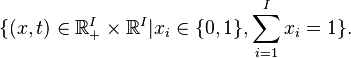
\{ (x,t)\in \mathbb{R}^I_+ \times \mathbb{R}^I | x_i \in \{0,1\} , \sum_{i=1}^I x_i = 1\}.

The x component describes the allocation of the object and t the transfers.

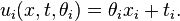
The buyer's types, or valuations of the object, are independent identically distributed random variables. A buyer of type $\theta_i$ has linear utility function u_i over the set of outcomes (the theorem also holds for the more general quasilinear utility functions):

u_i(x, t, \theta_i) = \theta_i x_i + t_i.

Thus an auction is a Bayesian game in which a player's strategy is his bid as a function of his type. An auction (more generally, a mechanism) is said to be Bayesian incentive compatible if all players bidding their true type is a Bayesian Nash equilibrium strategy profile.

Under these assumptions, the Revenue Equivalence Theorem then says the following:

Theorem For any two Bayesian incentive compatible auctions, if under their respective Bayesian Nash equilibria where all players bid their type,

a buyer of type θ_i has the same probability of getting the object across auctions, and
a buyer of lowest type has the same expected utility across auctions,

then the total expected transfers E_θ(Σt_i), i.e. the auctioneer's expected revenue, is the same for the two auctions.

In other words, if a buyer of given type has the same expected utility in the two auctions in the interim stage, then the seller's expected revenues are the same. However, ex post, the two mechanisms need not implement the same social choice functions. Two such examples are the second price auction and first price auction. Assume the types are drawn independently from the uniform distribution on [0,1]. In the second price auction, bidding one's own type is a dominant strategy, therefore a fortiori the auction is Bayesian incentive compatible. For the first price auction, it can be shown that the bid functions

b_i(\theta) = \frac{I-1}{I}(\theta^{I-1})

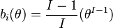
form a Bayesian Nash equilibrium (a simple argument via the revelation principle shows it can be made Bayesian incentive compatible). Thus the Revenue Equivalence Theorem applies: in both auctions, the highest types get the object and a buyer of type 0 has zero expected interim utility. They do not implement the same social choice functions.

Equivalence of Auction Mechanisms in Single Item Auctions

In fact, we can use revenue equivalence to prove that many types of auctions are revenue equivalent. For example, the first price auction, second price auction, and the all pay auction are all revenue equivalent.

Second Price Auction

Consider the second price single item auction, in which the player with the highest bid pays the second highest bid. It is optimal for each player $i$ to bid her own value $b_i=v_i$ .

Suppose $i$ wins the auction, and pays the second highest bid, or $\max_{j \neq i} b_j$ . The revenue from this auction is simply $\max_{j \neq i} b_j$ .

First Price Auction

In the first price auction, where the player with the highest bid simply pays her bid, if all players bid using a bidding function 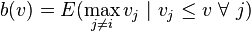$b(v) = E(\max_{j \neq i} v_j ~ | ~ v_j \le v ~ \forall ~ j)$ , this is a Nash equilibrium.

In other words, if each player bids such that they bid the expected value of second highest bid, assuming that theirs was the highest, then no player has any incentive to deviate. If this were true, then it is easy to see that the expected revenue from this auction is also $\max_{j \neq i} b_j$ if $i$ wins the auction.

Proof

To prove this, suppose that a player 1 bids $b(z) < v$ , effectively bluffing that her value is $z$ rather than $v$ . We want to find a value of $z$ such that the player's expected payoff is maximized.

The probability of winning is then 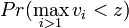$Pr(\max_{i > 1} v_i < z)$ . The expected cost of this bid is 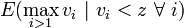$E(\max_{i>1} v_i~|~v_i<z~\forall~i)$ . Then a player's expected payoff is

Pr(\max_{i > 1} v_i < z)(v-E(\max_{i>1} v_i~|~v_i<z~\forall~i))

Let $X=\max_{i > 1} v_i$ , a random variable. Then we can rewrite the above as

Pr(X < z)(v-E(X~|X \le z))

Using the general fact that $E(X~|~X\le z)\cdot Pr(X<z) = \int_0^\infty Pr(X<z) - Pr(X<y)dy$ , we can rewrite the above as

Pr(X<z)\cdot v - Pr(X<z) \cdot z + \int_0^z Pr(X < y)dy

Taking derivatives with respect to $z$ , we obtain

Pr(X<z)'(v-z)=0 \Rightarrow v = z

Thus bidding with your value $v$ maximizes the player's expected payoff. Since $Pr(X<z)$ is monotone increasing, we verify that this is indeed a maximum point.

Using Revenue Equivalence to Predict Bidding Functions

We can use revenue equivalence to predict the bidding function of a player in a game. Consider the two player version of the second price auction and the first price auction, where each player's value is drawn uniformly from $[0,1]$ .

Second Price Auction

The expected payment of the first player in the second price auction can be computed as follows:

E(\text{Payment}~|~\text{Player 1 wins})P(\text{Player 1 wins}) + E(\text{Payment}~|~\text{Player 1 loses})P(\text{Player 1 loses})

Since players bid truthfully in a second price auction, we can replace all prices with players' values. If player 1 wins, he pays what player 2 bids, or $p_2=v_2$ . Player 1 himself bids $p_1=v_1$ . Since payment is zero when player 1 loses, the above is

E(v_2~|~v_2 < v_1)P(v_2 < v_1) + 0

Since $v_1,v_2$ come from a uniform distribution, we can simplify this to

\frac{v_1}{2} \cdot v_1 = \frac{v_1^2}{2}

First Price Auction

We can use revenue equivalence to generate the correct symmetric bidding function in the first price auction. Suppose that in the first price auction, each player has the bidding function $b(v)$ , where this function is unknown at this point.

The expected payment of player 1 in this game is then

E(\text{Payment}~|~\text{Player 1 wins})P(\text{Player 1 wins}) + E(\text{Payment}~|~\text{Player 1 loses})P(\text{Player 1 loses})

(as above)

Now, a player simply pays what the player bids, and let's assume that players with higher values still win, so that the probability of winning is simply a player's value, as in the second price auction. We will later show that this assumption was correct. Again, a player pays nothing if he loses the auction. We then obtain

b(v_1) \cdot v_1 + 0

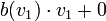
and by revenue equivalence,

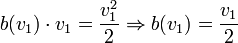
b(v_1) \cdot v_1 = \frac{v_1^2}{2} \Rightarrow b(v_1) = \frac{v_1}{2}

Indeed, with this bidding function, the player with the higher value still wins. We can also show that this is the correct equilibrium bidding function, by thinking about how a player should maximize his bid given that all other players are bidding using this bidding function.

All-pay Auctions

Similarly, we know that the expected payment of player 1 in the second price auction is $\frac{v_1^2}{2}$ , and this must be equal to the expected payment in the all-pay auction, i.e.

\frac{v_1^2}{2} = b(v_1)

Thus, the bidding function for each player in the all-pay auction is $\frac{v^2}{2}$

Revenue equivalence