Refinable function
In mathematics, in the area of wavelet analysis, a refinable function is a function which fulfils some kind of self-similarity. A function  is called refinable with respect to the mask
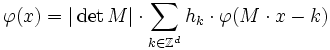
  if
if
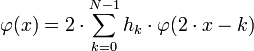
This condition is called refinement equation, dilation equation or two-scale equation.
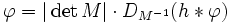
Using the convolution (denoted by a star, *) of a function with a discrete mask and the dilation operator  one can write more concisely:
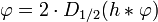
It means that one obtains the function, again, if you convolve the function with a discrete mask and then scale it back. There is a similarity to iterated function systems and de Rham curves.
The operator 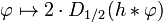 is linear.
A refinable function is an eigenfunction of that operator.
Its absolute value is not uniquely defined.
That is, if is a refinable function,
then for every
is linear.
A refinable function is an eigenfunction of that operator.
Its absolute value is not uniquely defined.
That is, if is a refinable function,
then for every  the function
  is refinable, too.
These functions play a fundamental role in wavelet theory as scaling functions.
Properties
Values at integral points
A refinable function is defined only implicitly.
It may also be that there are several functions which are refinable with respect to the same mask.
If shall have finite support
and the function values at integer arguments are wanted,
then the two scale equation becomes a system of simultaneous linear equations.
Let  be the minimum index and
  be the maximum index
of non-zero elements of , then one obtains
be the maximum index
of non-zero elements of , then one obtains
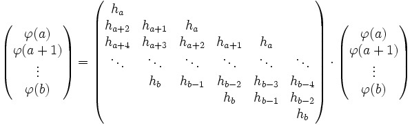 .
.
Using the discretization operator, call it  here, and the transfer matrix of , named
  , this can be written concisely as
 .
.
This is again a fixed-point equation.
But this one can now be considered as an eigenvector-eigenvalue problem.
That is, a finitely supported refinable function exists only (but not necessarily),
if has the eigenvalue 1.
Values at dyadic points
From the values at integral points you can derive the values at dyadic points,
i.e. points of the form  , with
  and
and  .
.

The star denotes the convolution of a discrete filter with a function.
With this step you can compute the values at points of the form  .
By replacing iteratedly by
.
By replacing iteratedly by  you get the values at all finer scales.

Convolution
If is refinable with respect to ,
and  is refinable with respect to
  ,
then
,
then  is refinable with respect to
  .
.
Differentiation
If is refinable with respect to ,
and the derivative  exists,
then is refinable with respect to
exists,
then is refinable with respect to  .
This can be interpreted as a special case of the convolution property,
where one of the convolution operands is a derivative of the Dirac impulse.
.
This can be interpreted as a special case of the convolution property,
where one of the convolution operands is a derivative of the Dirac impulse.
Integration
If is refinable with respect to ,
and there is an antiderivative  with
with
 ,
then the antiderivative
,
then the antiderivative 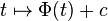 is refinable with respect to mask
  where the constant must fulfill
 .
.
If has bounded support,
then we can interpret integration as convolution with the Heaviside function and apply the convolution law.
Scalar products
Computing the scalar products of two refinable functions and their translates can be broken down to the two above properties.
Let  be the translation operator. It holds

where  is the adjoint of with respect to convolution,
i.e. is the flipped and complex conjugated version of ,
i.e.
is the adjoint of with respect to convolution,
i.e. is the flipped and complex conjugated version of ,
i.e. 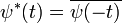 .
.
Because of the above property,  is refinable with respect to
  ,
and its values at integral arguments can be computed as eigenvectors of the transfer matrix.
This idea can be easily generalized to integrals of products of more than two refinable functions.[1]
,
and its values at integral arguments can be computed as eigenvectors of the transfer matrix.
This idea can be easily generalized to integrals of products of more than two refinable functions.[1]
Smoothness
A refinable function usually has a fractal shape. The design of continuous or smooth refinable functions is not obvious. Before dealing with forcing smoothness it is necessary to measure smoothness of refinable functions. Using the Villemoes machine[2] one can compute the smoothness of refinable functions in terms of Sobolev exponents.
In a first step the refinement mask is divided into a filter , which is a power of the smoothness factor  (this is a binomial mask) and a rest
  .
Roughly spoken, the binomial mask makes smoothness and
represents a fractal component, which reduces smoothness again.
Now the Sobolev exponent is roughly
the order of minus logarithm of the spectral radius of
.
Roughly spoken, the binomial mask makes smoothness and
represents a fractal component, which reduces smoothness again.
Now the Sobolev exponent is roughly
the order of minus logarithm of the spectral radius of  .
.
Generalization
The concept of refinable functions can be generalized to functions of more than one variable,
that is functions from  .
The most simple generalization is about tensor products.
If and are refinable with respect to and , respectively, then
.
The most simple generalization is about tensor products.
If and are refinable with respect to and , respectively, then  is refinable with respect to
  .
.
The scheme can be generalized even more to different scaling factors with respect to different dimensions or even to mixing data between dimensions.[3]
Instead of scaling by scalar factor like 2 the signal the coordinates are transformed by a matrix  of integers.
In order to let the scheme work, the absolute values of all eigenvalues of must be larger than one.
(Maybe it also suffices that
of integers.
In order to let the scheme work, the absolute values of all eigenvalues of must be larger than one.
(Maybe it also suffices that 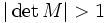 .)
.)
Formally the two-scale equation does not change very much:
Examples
- If the definition is extended to distributions, then the Dirac impulse is refinable with respect to the unit vector
 , that is known as Kronecker delta. The
  -th derivative of the Dirac distribution is refinable with respect to
  .
. - The Heaviside function is refinable with respect to
 .
. - The truncated power functions with exponent are refinable with respect to
 .
. - The triangular function is a refinable function.[4] B-Spline functions with successive integral nodes are refinable, because of the convolution theorem and the refinability of the characteristic function for the interval
 (a boxcar function).
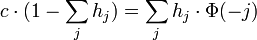
 - All polynomial functions are refinable. For every refinement mask there is a polynomial that is uniquely defined up to a constant factor. For every polynomial of degree there are many refinement masks that all differ by a mask of type
 for any mask
  and the convolutional power
  .[5]
.[5] - A rational function is refinable if and only if it can be represented using partial fractions as
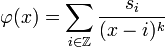 , where
  is a positive natural number and
  is a real sequence with finitely many non-zero elements (a Laurent polynomial) such that
  (read:
 ![\exists h(z)\in\mathbb{R}[z,z^{-1}]\ h(z)\cdot s(z) = s(z^2)](../I/m/5d312fe2c3fdf9b1c0d13e62d74ac8cd.png) ). The Laurent polynomial
). The Laurent polynomial  is the associated refinement mask.[6]
References
- ↑ Dahmen, Wolfgang; Micchelli, Charles A. (1993). "Using the refinement equation for evaluating integrals of wavelets". Journal Numerical Analysis (SIAM) 30: 507–537.
- ↑ Villemoes, Lars. "Sobolev regularity of wavelets and stability of iterated filter banks" (POSTSCRIPT). Retrieved 2006.
- ↑ Berger, Marc A.; Wang, Yang (1992), "Multidimensional two-scale dilation equations (chapter IV)", in Chui, Charles K., Wavelet Analysis and its Applications 2, Academic Press, Inc., pp. 295–323 Missing or empty
|title=(help) - ↑ Nathanael, Berglund. "Reconstructing Refinable Functions". Retrieved 2010-12-24.
- ↑ Thielemann, Henning (2012-01-29). "How to refine polynomial functions". arXiv:1012.2453.
- ↑ Gustafson, Paul; Savir, Nathan; Spears, Ely (2006-11-14), "A Characterization of Refinable Rational Functions" (PDF), American Journal of Undergraduate Research 5 (3): 11–20