Rayleigh–Ritz method

The Rayleigh–Ritz method (after Walther Ritz and Lord Rayleigh) is a widely used method used to approximate eigenvalues and eigenvectors. In this method the expression for a variable which depends upon max 3 or 4 variables are used. If the number of independent variables become more than 4 then it is very difficult to find expression for dependent variables.

Description of method

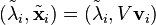
The Rayleigh–Ritz method allows for the computation of Ritz pairs $(\tilde{\lambda}_i,\tilde{\textbf{x}}_i)$ which approximate the solutions to the eigenvalue problem ^[1]

A \textbf{x} = \lambda x

Where $A \in \mathbb{C}^{N \times N}$ .

The procedure is as follows:^[2]

Compute an orthonormal basis $V \in \mathbb{C}^{N \times m}$ approximating the eigenspace corresponding to m eigenvectors
Compute $R \gets V^* A V$
Compute the eigenvalues of R solving $R \mathbf{v}_i = \tilde{\lambda}_i \mathbf{v}_i$
Form the ritz pairs $(\tilde{\lambda}_i,\tilde{\textbf{x}}_i) = (\tilde{\lambda}_i,V \textbf{v}_i)$

One can always compute the accuracy of such an approximation via 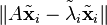$\| A \tilde{\textbf{x}}_i - \tilde{\lambda}_i \tilde{\textbf{x}}_i\|$

If a Krylov subspace is used and A is a general matrix, then this is the Arnoldi Algorithm.

Example: Mechanical Engineering

Typically in mechanical engineering it is used for finding the approximate real resonant frequencies of multi degree of freedom systems, such as spring mass systems or flywheels on a shaft with varying cross section. It is an extension of Rayleigh's method. It can also be used for finding buckling loads and post-buckling behaviour for columns.

The following discussion uses the simplest case, where the system has two lumped springs and two lumped masses, and only two mode shapes are assumed. Hence M = [m₁, m₂] and K = [k₁, k₂].

A mode shape is assumed for the system, with two terms, one of which is weighted by a factor B, e.g. Y = [1, 1] + B[1, −1]. Simple harmonic motion theory says that the velocity at the time when deflection is zero, is the angular frequency $\omega$ times the deflection (y) at time of maximum deflection. In this example the kinetic energy (KE) for each mass is $\frac{1}{2}\omega^2 Y_1^2 m_1$ etc., and the potential energy (PE) for each spring is $\frac{1}{2} k_1 Y_1^2$ etc. For continuous systems the expressions are more complex.

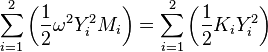
We also know, since no damping is assumed, that KE when y=0 equals the PE when v=0 for the whole system. As there is no damping all locations reach v=0 simultaneously.

so, since KE = PE,

\sum_{i=1}^2 \left(\frac{1}{2} \omega^2 Y_i^2 M_i\right)=\sum_{i=1}^2 \left(\frac{1}{2} K_i Y_i^2\right)

Note that the overall amplitude of the mode shape cancels out from each side, always. That is, the actual size of the assumed deflection does not matter, just the mode shape.

Mathematical manipulations then obtain an expression for $\omega$ , in terms of B, which can be differentiated with respect to B, to find the minimum, i.e. when $d\omega/dB=0$ . This gives the value of B for which $\omega$ is lowest. This is an upper bound solution for $\omega$ if $\omega$ is hoped to be the predicted fundamental frequency of the system because the mode shape is assumed, but we have found the lowest value of that upper bound, given our assumptions, because B is used to find the optimal 'mix' of the two assumed mode shape functions.

There are many tricks with this method, the most important is to try and choose realistic assumed mode shapes. For example in the case of beam deflection problems it is wise to use a deformed shape that is analytically similar to the expected solution. A quartic may fit most of the easy problems of simply linked beams even if the order of the deformed solution may be lower. The springs and masses do not have to be discrete, they can be continuous (or a mixture), and this method can be easily used in a spreadsheet to find the natural frequencies of quite complex distributed systems, if you can describe the distributed KE and PE terms easily, or else break the continuous elements up into discrete parts.

This method could be used iteratively, adding additional mode shapes to the previous best solution, or you can build up a long expression with many Bs and many mode shapes, and then differentiate them partially.

Notes

↑ Trefethen and Bau (1997), pg. 254
↑ G. Schofield, J. R. Chelikowsky, Y. Saad (2011). pg 6

References

Trefethen L, Bau D. Numerical Linear Algebra. SIAM 1997
G. Schofield, J. R. Chelikowsky, and Yousef Saad.

A spectrum slicing method for the kohn-sham problem. Preprint umsi-2011-142, Minnesota Supercomputer Institute, University of Minnesota, Minneapolis, MN, 2011

External links

http://www.math.nps.navy.mil/~bneta/4311.pdf - Course on Calculus of Variations, has a section on Rayleigh–Ritz method.