Rao–Blackwell theorem

In statistics, the Rao–Blackwell theorem, sometimes referred to as the Rao–Blackwell–Kolmogorov theorem, is a result which characterizes the transformation of an arbitrarily crude estimator into an estimator that is optimal by the mean-squared-error criterion or any of a variety of similar criteria.

The Rao–Blackwell theorem states that if g(X) is any kind of estimator of a parameter θ, then the conditional expectation of g(X) given T(X), where T is a sufficient statistic, is typically a better estimator of θ, and is never worse. Sometimes one can very easily construct a very crude estimator g(X), and then evaluate that conditional expected value to get an estimator that is in various senses optimal.

The theorem is named after Calyampudi Radhakrishna Rao and David Blackwell. The process of transforming an estimator using the Rao–Blackwell theorem is sometimes called Rao–Blackwellization. The transformed estimator is called the Rao–Blackwell estimator.

Definitions

An estimator δ(X) is an observable random variable (i.e. a statistic) used for estimating some unobservable quantity. For example, one may be unable to observe the average height of all male students at the University of X, but one may observe the heights of a random sample of 40 of them. The average height of those 40—the "sample average"—may be used as an estimator of the unobservable "population average".

A sufficient statistic T(X) is a statistic calculated from data X to estimate some parameter θ for which it is true that no other statistic which can be calculated from data X provides any additional information about θ. It is defined as an observable random variable such that the conditional probability distribution of all observable data X given T(X) does not depend on the unobservable parameter θ, such as the mean or standard deviation of the whole population from which the data X was taken. In the most frequently cited examples, the "unobservable" quantities are parameters that parametrize a known family of probability distributions according to which the data are distributed.

In other words, a sufficient statistic T(X) for a parameter θ is a statistic such that the conditional distribution of the data X, given T(X), does not depend on the parameter θ.

A Rao–Blackwell estimator δ₁(X) of an unobservable quantity θ is the conditional expected value E(δ(X) | T(X)) of some estimator δ(X) given a sufficient statistic T(X). Call δ(X) the "original estimator" and δ₁(X) the "improved estimator". It is important that the improved estimator be observable, i.e. that it not depend on θ. Generally, the conditional expected value of one function of these data given another function of these data does depend on θ, but the very definition of sufficiency given above entails that this one does not.

The mean squared error of an estimator is the expected value of the square of its deviation from the unobservable quantity being estimated.

The theorem

Mean-squared-error version

One case of Rao–Blackwell theorem states:

The mean squared error of the Rao–Blackwell estimator does not exceed that of the original estimator.

In other words

\operatorname{E}((\delta_1(X)-\theta)^2)\leq \operatorname{E}((\delta(X)-\theta)^2).\,\!

The essential tools of the proof besides the definition above are the law of total expectation and the fact that for any random variable Y, E(Y²) cannot be less than [E(Y)]². That inequality is a case of Jensen's inequality, although it may also be shown to follow instantly from the frequently mentioned fact that

0 \leq \operatorname{Var}(Y) = \operatorname{E}((Y-\operatorname{E}(Y))^2) = \operatorname{E}(Y^2)-(\operatorname{E}(Y))^2.\,\!

Convex loss generalization

The more general version of the Rao–Blackwell theorem speaks of the "expected loss" or risk function:

\operatorname{E}(L(\delta_1(X)))\leq \operatorname{E}(L(\delta(X)))\,\!

where the "loss function" L may be any convex function. For the proof of the more general version, Jensen's inequality cannot be dispensed with.

Properties

The improved estimator is unbiased if and only if the original estimator is unbiased, as may be seen at once by using the law of total expectation. The theorem holds regardless of whether biased or unbiased estimators are used.

The theorem seems very weak: it says only that the Rao–Blackwell estimator is no worse than the original estimator. In practice, however, the improvement is often enormous.

Example

Phone calls arrive at a switchboard according to a Poisson process at an average rate of λ per minute. This rate is not observable, but the numbers X₁, ..., X_n of phone calls that arrived during n successive one-minute periods are observed. It is desired to estimate the probability e^−λ that the next one-minute period passes with no phone calls.

An extremely crude estimator of the desired probability is

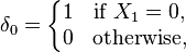
\delta_0=\left\{\begin{matrix}1 & \text{if}\ X_1=0, \\ 0 & \text{otherwise,}\end{matrix}\right.

i.e., it estimates this probability to be 1 if no phone calls arrived in the first minute and zero otherwise. Despite the apparent limitations of this estimator, the result given by its Rao–Blackwellization is a very good estimator.

The sum

S_n = \sum_{i=1}^n X_{i} = X_1+\cdots+X_n\,\!

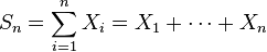
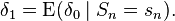
can be readily shown to be a sufficient statistic for λ, i.e., the conditional distribution of the data X₁, ..., X_n, depends on λ only through this sum. Therefore, we find the Rao–Blackwell estimator

\delta_1=\operatorname{E}(\delta_0\mid S_n=s_n).

After doing some algebra we have

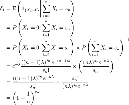
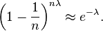
\begin{align} \delta_1 &= \operatorname{E} \left (\mathbf{1}_{\{X_1=0\}} \Bigg| \sum_{i=1}^n X_{i} = s_n \right ) \\ &= P \left (X_{1}=0 \Bigg| \sum_{i=1}^n X_{i} = s_n \right ) \\ &= P \left (X_{1}=0, \sum_{i=2}^n X_{i} = s_n \right ) \times P \left (\sum_{i=1}^n X_{i} = s_n \right )^{-1} \\ &= e^{-\lambda}\frac{\left((n-1)\lambda\right)^{s_n}e^{-(n-1)\lambda}}{s_n!} \times \left (\frac{(n\lambda)^{s_n}e^{-n\lambda}}{s_n!} \right )^{-1} \\ &= \frac{\left((n-1)\lambda\right)^{s_n}e^{-n\lambda}}{s_n!} \times \frac{s_n!}{(n\lambda)^{s_n}e^{-n\lambda}} \\ &= \left(1-\frac{1}{n}\right)^{s_n} \end{align}

Since the average number of calls arriving during the first n minutes is nλ, one might not be surprised if this estimator has a fairly high probability (if n is big) of being close to

\left(1-{1 \over n}\right)^{n\lambda}\approx e^{-\lambda}.

So δ₁ is clearly a very much improved estimator of that last quantity. In fact, since S_n is complete and δ₀ is unbiased, δ₁ is the unique minimum variance unbiased estimator by the Lehmann–Scheffé theorem.

Idempotence

The Rao–Blackwell process is idempotent. Using it to improve the already improved estimator does not obtain a further improvement, but merely returns as its output the same improved estimator.

Completeness and Lehmann–Scheffé minimum variance

If the conditioning statistic is both complete and sufficient, and the starting estimator is unbiased, then the Rao–Blackwell estimator is the unique "best unbiased estimator": see Lehmann–Scheffé theorem.

References

Blackwell, D. (1947). "Conditional expectation and unbiased sequential estimation". Annals of Mathematical Statistics 18 (1): 105–110. doi:10.1214/aoms/1177730497. MR 19903. Zbl 0033.07603.
Kolmogorov, A. N. (1950). "Unbiased estimates". Izvestiya Akad. Nauk SSSR. Ser. Mat. 14: 303–326. MR 36479.

Radhakrishna Rao, C. "Information and accuracy attainable in the estimation of statistical parameters." Bulletin of the Calcutta Mathematical Society 37, no. 3 (1945): 81-91.

External links

Nikulin, M.S. (2001), "Rao–Blackwell–Kolmogorov theorem", in Hazewinkel, Michiel, Encyclopedia of Mathematics, Springer, ISBN 978-1-55608-010-4