Rabi cycle
A great variety of physical processes belonging to the areas of quantum computing, condensed matter, atomic and molecular physics, and nuclear and particle physics can be conveniently studied in terms of two-level quantum mechanical systems. In this case, one of the effects is represented by the oscillations between the two energy levels, as for example, electron neutrino ν
e − muon neutrino ν
μ flavour neutrino oscillations. In physics, the Rabi cycle is the cyclic behaviour of a two-state quantum system in the presence of an oscillatory driving field. A two-state system has two possible states, and if they are not degenerate (i.e. equal energy), the system can become "excited" when it absorbs a quantum of energy.
The effect is important in quantum optics, nuclear magnetic resonance and quantum computing. The term is named in honour of Isidor Isaac Rabi.
When an atom (or some other two-level system) is illuminated by a coherent beam of photons, it will cyclically absorb photons and re-emit them by stimulated emission. One such cycle is called a Rabi cycle and the inverse of its duration the Rabi frequency of the photon beam.
This mechanism is fundamental to quantum optics. It can be modeled using the Jaynes-Cummings model and the Bloch vector formalism.
For example, for a two-state atom (an atom in which an electron can either be in the excited or ground state) in an electromagnetic field with frequency tuned to the excitation energy, the probability of finding the atom in the excited state is found from the Bloch equations to be:
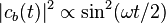 ,
,
where  is the Rabi frequency.
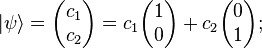
More generally, one can consider a system where the two levels under consideration are not energy eigenstates. Therefore if the system is initialized in one of these levels, time evolution will make the population of each of the levels oscillate with some characteristic frequency, whose angular frequency[1] is also known as the Rabi frequency. The state of a two-state quantum system can be represented as vectors of a two-dimensional complex Hilbert space, which means every state vector  is represented by two complex coordinates.
 where
where  and
and  are the coordinates.[2]
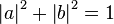
If the vectors are normalized, and are related by 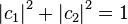 . The basis vectors will be represented as
  and
and 
All observable physical quantities associated with this systems are 2  2 Hermitian matrices, which means the Hamiltonian of the system is also a similar matrix.
How to prepare an oscillation experiment in a quantum system
One can construct an oscillation experiment consisting of following steps:[3]
(1)Prepare the system in a fixed state say 
(2)Let the state evolve freely, under a Hamiltonian H for time t
(3)Find the probability P(t), that the state is in
If was an eigenstate of H, P(t)=1 and there are no oscillations. Also if two states are degenerate, every state including is an eigenstate of H. As a result there are no oscillations. So if H has no degenerate eigenstates, neither of which is , then there will be oscillations. These probabilities of oscillations are given by Rabi Formula. Oscillations between two levels are called Rabi oscillation. The most general form of the Hamiltonian of a two-state system is given
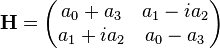
here,  and
and  are real numbers. This matrix can be decomposed as,

The matrix  is the 2 2 identity matrix and the matrices
 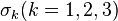 are the Pauli matrices. This decomposition simplifies the analysis of the system especially in the time-independent case where the values of and are constants. Consider the case of a spin-1/2 particle in a magnetic field
  . The interaction Hamiltonian for this system is
 .Where
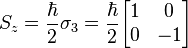
where  is the magnitude of the particle's magnetic moment,
 is Gyromagnetic ratio and
  is the vector of Pauli matrices. Here eigenstates of Hamiltonian are eigenstates of
  that is and
  . The probability that a system in the state
  will be found to be in the arbitrary state
  is given by
  . Let system initially
  is in state
  that is eigen state of
  ,
,
 . That is
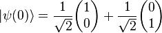 . Here Hamiltonian is time independent. So by solving time independent Schrödinger equation, we get state after time t is given by
 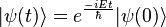 , where E is the total energy of system. So the state after time t is given by
 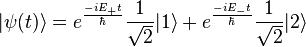 . Now suppose spin is measured in the x-direction at time t, the probability of finding spin-up is given by
  where is a characteristic angular frequency given by
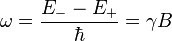 where it has been assumed that
  .[4] So in this case probability of finding spin up state in X direction is oscillatory in time t when system is initially in Z direction. Similarly if we measure spin in Z direction then probability of finding
  of the system is
  .In the case
  , that is when the Hamiltonian is degenerate there is no oscillation. So we can conclude that if the eigenstate of an above given Hamiltonian represents the state of a system, then probability of the system being that state is not oscillatory, but if we find probability of finding the system in other state, it is oscillatory. This is true for even time dependent Hamiltonian. For example
 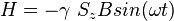 , the probability that a measurement of system in Y direction at time t results in
  is
is 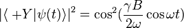 , where initial state is in
  .[5]
.[5]
Example of Rabi Oscillation between two states in ionized hydrogen molecule. Ionized hydrogen molecule is composed of two proton  and
and  and one electron. The two protons because of their large masses can be considered to be fixed. Let us call R be the distance between them and and the states where the electron is localised around or. Assume, at a certain time, the electron is localised about proton . According to the results of previous section we know it will oscillate between the two protons with a frequency equal to the Bohr frequency associated with two stationary state
  and
and  of molecule.
This oscillation of the electron between the two states corresponds to an oscillation of the mean value of the electric dipole moment of the molecule. Thus when the molecule is not in a stationary state, an oscillating electric dipole moment can appear. Such an oscillating dipolemoment can exchange energy with an electromagnetic wave of same frequency. Consequently, this frequency must appear in the absorption and emission spectrum of Ionized hydrogen molecule.
Derivation of Rabi Formula in an Nonperturbative Procedure by means of the Pauli matrices
Let us consider a Hamiltonian in the form  .
.
The eigen values of this matrix are given by  and
and  .Where
  and
and  . so we can take
  .
.
Now eigen vector for  can be found from equation :
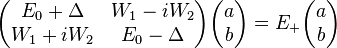 .
.
So 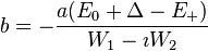 .
.
Using normalisation condition of eigen vector,
 .So
.So 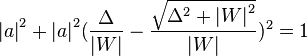 .
.
Let 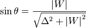 and
and 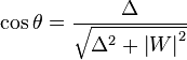 . so
. so 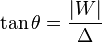 .
.
So we get 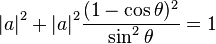 . That is
 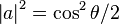 . Taking arbitrary phase angle
  ,we can write
 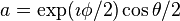 . Similarly
 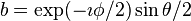 .
.
So eigen vector for eigen value is given by 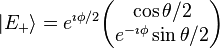 .
.
As overall phase is immaterial so we can write 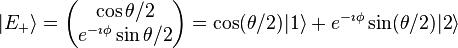 .
.
Similarly we can find eigen vector for  value and we get
  .
.
From these two equations, we can write  and
and  .
.
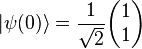
Let at time t=0, system be in That Is  .
.
State of system after time t is given by  .
.
Now a system is in one of the eigen states or , it will remain the same state, however in a general state as shown above the time evolution is non trivial.
The probability amplitude of finding the system at time t in the state is given by  .
.
Now the probability that a system in the state  will be found to be in the arbitrary state is given by
By simplifying  .........(1).
This shows that there is a finite probability of finding the system in state when the system is originally in the state . The probability is oscillatory with angular frequency 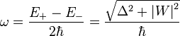 , which is simply unique Bohr frequency of the system and also called Rabi frequency. The formula(1) is known as Rabi formula. Now after time t the probability that the system in state is given by
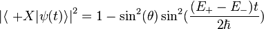 , which is also oscillatory. This type of oscillations between two levels are called Rabi oscillation and seen in many problems such as Neutrino oscillation, ionized Hydrogen molecule, Quantum computing, Ammonia maser etc.
Rabi oscillation in Quantum computing
Any two state system is called qubit. Let a Spin half system be placed in a classical magnetic field with periodic component such as  . The Hamiltonian of system (proton) of magnetic moment in field
 is given
  , where
  and b
and b  ,
, is gyromagnetic ratio of proton. One can find eigen value and eigen vector of the Hamiltonian by above mentioned procedure. Let at time t=0 the qubit is in the state, at time t it will have a probability
  of being found in state given by
 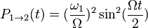 where
where 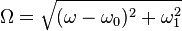 . This is the phenomenon of Rabi oscillation. The oscilltion between the levels and has maximum amplitude for
  that is at resonance. So
 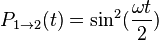 . To go from state to state it is sufficient to adjust the time t during which the rotating field acts such as
  or
or  . This is called a
  pulse. If a time intermediate between 0 and
  is chosen, we obtain a superposition of and . In particular
  , we have a
  pulse:
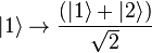 . This operation has crucial importance in quantum computing. The equations are essentially identical in the case of a two level atom in the field of a laser when the generally well satisfied rotating wave approximation is made.Then
  is the energy difference between the two atomic levels, is the frequency of laser wave and Rabi frequency
  is proportional to the product of the transition electric dipole moment of atom
  and electric field
  of the laser wave that is
  . In summary, Rabi oscillations are the basic process used to manipulate qubits. These oscillations are obtained by exposing qubits to periodic electric or magnetic fields during suitably adjusted time intervals.[6]
Rabi oscillation in Ammonia maser
In molecular physics, a well known example of a two-state system is a nitrogen atom in the double-well potential of an ammonia molecule. The tunnel splitting of the ammonia NH3 molecule finds application in the ammonia MASER, an acronym for Microwave Amplification of Stimulated Emission of Radiation, similarly as LASER is an acronym for Light Amplification. While magnetic interactions of the NH3 molecules are negligible, the molecules’ dipolemoments are very sensitive to external electric fields. A prominent cause for the splitting of energy levels is the tunnel effect. As an example we regard the ammonia molecule NH3. If we squeeze the nitrogen atom along the z-axis through the equilateral triangle formed by the hydrogen atoms, then the N atom sees a double well potential V (z). The N atom can be on either side of the plane of the H-atoms. Hence the NH3 molecule forms a two-state system with two basis states or spatial eigenstates  and
and  with the nitrogen atom on one side or the other of the plane of hydrogen atoms, and its energy ground and first excited states and are the symmetric and antisymmetric quantum superpositions of the spatial eigenstates (ignoring rotational and vibrational states). The system can change from L to R and back because there is a certain probability amplitude A that the nitrogen atom tunnels through the central potential barrier to the other well. The ammonia maser is based upon the transition between the energy eigenstates, which may also be described as the Rabi oscillation between the spatial eigenstates. However, the inversion transition is seen only at low gas pressure. As the gas pressure is increased, the transition broadens, shifts to lower frequency and then quenches (the frequency goes to zero). The ammonia molecule appears to undergo spatial localisation as a result of interaction with the environment. This would be of immense theoretical interest. In chemistry and in the classical world generally, enantiomorphic molecules with distinguishable spatial eigenstates and are always found in their spatial eigenstates (classical behaviour) rather than their energy ground states (quantum behaviour). Whilst ammonia is not enantiomorphic, it does appear to show both behaviours, quantum at low pressure and classical at high pressure, if the quenching is considered to be a direct observation of localisation or collapse of the wave-function into a spatial eigenstate. Within the context of the decoherence programme, it has been treated quantitatively in that way. The broadening, shift and quenching of the Rabi oscillation are simply consequences of impacts and may be described within the framework of an oscillator subject to white noise from the environment. There is no evidence for localisation onto spatial eigen states.[7]
See also
- Atomic coherence
- Bloch sphere
- Laser pumping
- Optical pumping
- Rabi problem
- Vacuum Rabi oscillation
- Neutral particle oscillation
References
- ↑ Encyclopedia of Laser Physics and Technology - Rabi oscillations, Rabi frequency, stimulated emission
- ↑ Griffiths, David (2005). Introduction to Quantum Mechanics (2nd ed.). p. 353.
- ↑ Sourendu Gupta (27 August 2013). "The physics of 2-state systems" (PDF). Tata Institute of Fundamental Research.
- ↑ Griffiths, David (2012). Introduction to Quantum Mechanics (2nd ed.) p. 191.
- ↑ Griffiths, David (2012). Introduction to Quantum Mechanics (2nd ed.) p. 196 ISBN 978-8177582307
- ↑ A Short Introduction to Quantum Information and Quantum Computation by Michel Le Bellac, ISBN 978-0521860567
- ↑ "au:Herbauts_I in:quant-ph - SciRate Search". SciRate.
- Quantum Mechanics Volume 1 by C. Cohen-Tannoudji, Bernard Diu, Frank Laloe, ISBN 9780471164333
- A Short Introduction to Quantum Information and Quantum Computation by Michel Le Bellac, ISBN 978-0521860567
- The Feynman Lectures on Physics Vol 3 by Richard P. Feynman & R.B. Leighton, ISBN 978-8185015842
- Modern Approach To Quantum Mechanics by John S Townsend, ISBN 9788130913148