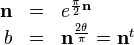
Quaternion rotation biradial
In mathematics, a quaternion biradial[1](Art.93) is the quotient (or product  ,
,  ,
,  ,
,  ) of two pure quaternion vectors
  and
and  , sometimes called rays.
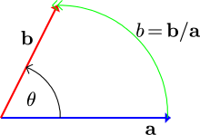
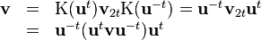
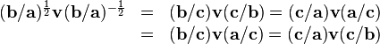
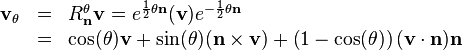
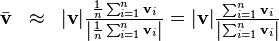
Consider the quaternion biradial  (read “b by a”). The biradial
  is an operator that turns into as an operator on :
  . The biradial turning operation is a composition of a rotation and a scaling that rotates into the line of , followed with scaling by
  . If
. If  then
then  and acts as only a rotation operator (a.k.a., a versor, rotor, or 2D spinor) in the -plane through the angle
  from to .
Quaternion spatial rotations explained using Hamilton’s biradial concept
Quaternion identities
For simplicity in the following explanations, let 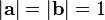 so that and are unit vectors. Frequent use will be made of the following identities.
Definition of quaternion units and products:
Unit vectors:
![\begin{array}{rcl}
\mathbf{u} & = & u_{x} \mathbf{i}+u_{y} \mathbf{j}+u_{z} \mathbf{k}=
\sin( \phi ) \left[ \cos( \theta ) \mathbf{i}+
\sin( \theta ) \mathbf{j} \right] + \cos( \phi )
\mathbf{k}\\
\mathbf{a}^{2} =\mathbf{b}^{2} =\mathbf{u}^{2} & = & u^{2}_{x}
\mathbf{i}^{2} +u^{2}_{y} \mathbf{j}^{2} +u^{2}_{z} \mathbf{k}^{2} +\\
& & u_{x} u_{y} ( \mathbf{i}\mathbf{j}+\mathbf{j}\mathbf{i} ) +u_{x} u_{z}
( \mathbf{i}\mathbf{k}+\mathbf{k}\mathbf{i} ) +u_{y} u_{z} (
\mathbf{j}\mathbf{k}+\mathbf{k}\mathbf{j} )\\
& = & -u_{x}^{2} -u_{y}^{2} -u_{z}^{2} =- | \mathbf{u} |^{2} =-1.\end{array}](../I/m/2d8e33110a628b19e7dd3d94202117c5.png)
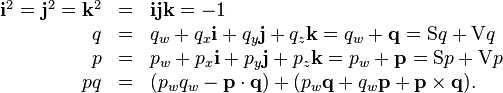
Conjugate, tensor, and versor operations:
Inverses of a quaternion and a vector:
Vector products:
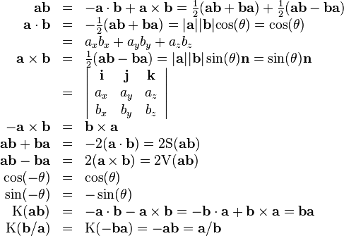
The operations  ,
,  ,
,  ,
,  ,
,  are the scalar part, vector part, conjugate, tensor, and versor of quaternion
  in Hamilton’s notation and terminology.
Since scalars commute with all elements in the quaternion algebra, so do scalars such as ,  ,
,  , and
, and  .
.
For perpendicular vectors  , and
, and  . Therefore,
  ,
,  , and
, and  .
.
For any scalar  and value
  where
where  , the Taylor series for
  gives the Euler formula

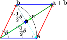
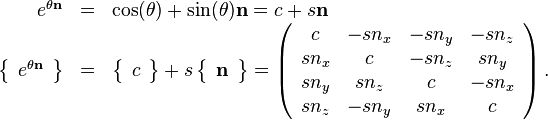
The biradial b/a
The biradial can be written
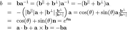
where  is the component of parallel to ,
  is the component of perpendicular to , is the angle from to , and
 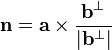 is the unit vector normal to the -plane.
Quadrantal versors and handedness
When  then
then  , showing that
  is the quadrantal versor of the -plane perpendicular to . We can also write
where is the number of quadrants (multiples of  radians) of rotation round as the axis of rotation following a right-hand rule on a right-handed axes model or following a left-hand rule on a left-handed axes model. If is at a positive angle in the plane from , this means that on right-handed axes,
  rotates by right-hand rule counter-clockwise from into , while on left-handed axes rotates by left-hand rule clockwise from into . Angles are positive counter-clockwise on right-handed axes, and are positive clockwise on left-handed axes. The choice of right-handed or left-handed axes is a modeling choice outside the algebra that affects the geometric interpretation of the algebra but not the algebra itself.
The relation between the unit vectors 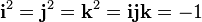 as defined by Hamilton, also defines
  as the quadrantal versors or biradials
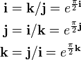
following a right-hand (counter-clockwise) rule on right-handed axes or a left-hand (clockwise) rule on left-handed axes, where  each rotate by
  radians in their perpendicular plane according to the matching handedness rule and axes model being used.
Quaternions and the left-hand rule on left-handed axes
In a sense, a left-hand rule and axes are a better fit to Hamilton’s defined relation since then a versor used as left-side multiplier to operate on a right-side multiplicand performs left-hand clockwise rotation for positive angles, and the same versor used as a right-side multiplier to operate on a left-side multiplicand performs right-hand counter-clockwise rotation by the same angle (the reverse rotation). For example, imagine working on left-handed axes and interpret the geometry represented by the following quadrantal versor rotations
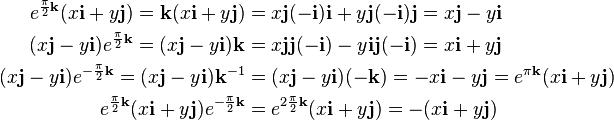
which show that operating with  on the left-side performs left-hand clockwise rotation, operating with on the right-side performs a right-hand counter-clockwise (reverse) rotation, and operating with
  on the right-side performs another clockwise rotation.
On left-handed axes, there is arguably more consistency of handedness as if the quaternion relation was defined for a left-handed system of axes. It is also possible for the relation to have been defined  , inverting the quaternion space and making right-handed axes arguably match the geometric interpretation of the algebra better. In Hamilton’s book Lectures on Quaternions[1] he often uses left-handed[1](Art.228) axes with left-hand rule clockwise rotations, and it seems that was often the preferred orientation used by the inventor of quaternions.
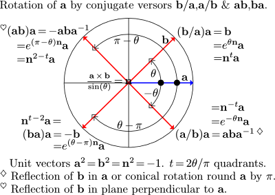
Rotation formulas
These results so far will be shown to generalize for any quadrantal versor  rotating a vector
  by
by  quadrants or by
  radians in the plane perpendicular to as
where for  quadrant the result is the reflection of in , or conically rotated
  round , or is conjugated by . Note that we need to convert angles in quadrants to radians since the ordinary trigonometric functions
  ,
,  are defined for in radians.
The scalar power of a vector
Any versor can be constructed or expressed using its rotational angle in quadrants and its unit vector or quadrantal versor rotational axis as  . This expression seems to be seldomly used but is important to understand since it gives a clear geometric meaning to taking the scalar power of a vector. For a general vector
  , its scalar power of can be expressed as
  and still represents a versor
  that rotates round
  by quadrants or radians, and also a scaling or tensor (in Hamilton’s terminology and notation)
  that is applied times.
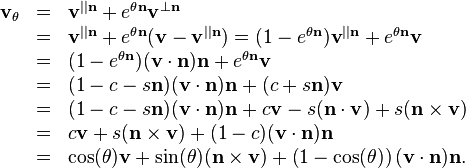
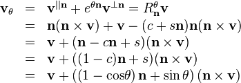
Rotation of vector components parallel and perpendicular to a rotation axis
When is a vector in the plane perpendicular to , then and are perpendicular and obey the anti-commutative multiplication property  , leading to
which demonstrates that the conjugate versor  applied as right-side operator on rotates the same (in the plane perpendicular to the versor axis ) as the versor itself applied as left-side operator on , and vice versa. The reverse rotation can be written
which is also seen as two successive rotations with the second outer rotation undoing or reversing the first inner rotation.
When is a vector parallel to , then their multiplication  is commutative, leading to

where is unaffected by the rotation.
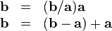
In general, a vector will be neither completely parallel nor perpendicular to another vector . Similar to how was written above in the expressions for , a vector can be written 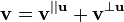 since it is always possible for any vector to be written as a sum of components parallel and perpendicular to any other vector . The parallel part
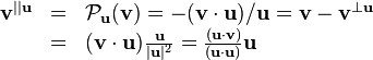
is the projection of on . The perpendicular part
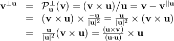
is the rejection of by . We can also write the orthogonalization of by as

Combining some results from above we get
which represents the component  unaffected by a null (or any) rotation round , while the component
  undergoes a planar rotation by
  in the plane perpendicular to . The sum of these vectors is the rotated version
  of . This is an important formula for the type of rotation known as conical rotation by round the line of relative to the origin. The cone apex is the origin, the cone base is in the plane perpendicular to and intersecting at distance
  from the origin, and the sides of the cone are swept by the line of as it is rotated round axis for a complete
  rotation.
A versor and its conjugate have the same angle but inverse axes
or they have the same axis but reverse angles
however, there is often a preference to take positive angles and inverse axes. The conjugate or inverse versor is sometimes also called the reversor of .
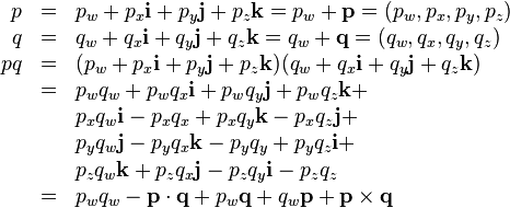
We’ve looked at the biradial already, so let’s now look at the other products.
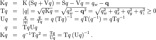
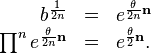
The product ba
The product gives
![\begin{array}{rcl}
\mathbf{b}\mathbf{a} & = & \mathbf{b}\mathbf{a}^{-1} \mathbf{a}^{2}
=\mathbf{a}^{2} \mathbf{b}\mathbf{a}^{-1} =-\mathbf{b}\mathbf{a}^{-1}\\
& = & e^{\pi \mathbf{n}} e^{\theta \mathbf{n}} =e^{( \pi + \theta )
\mathbf{n}}\\
& = & e^{( \pi + \theta -2 \pi ) \mathbf{n}} =e^{( \theta - \pi )
\mathbf{n}} =e^{( \pi - \theta ) ( -\mathbf{n} )}\\
& = & - \left[ \mathrm{cos} ( \theta ) + \sin ( \theta ) \mathbf{n}
\right] =-\mathbf{b} \cdot \mathbf{a}+\mathbf{b} \times \mathbf{a}=
\mathrm{K} ( \mathbf{a}\mathbf{b} )\end{array}](../I/m/1409e9993e3b0c5820026a1498cd1b2a.png)
showing that, compared to the quotient , the product rotates by an additional angle or an angle  round the same axis , or rotates by the supplement angle
  in the opposite direction round the inverse axis
  . Notice how multiplying by
  is the same as rotating by an additional
  round the same axis.
The biradial a/b
The biradial gives
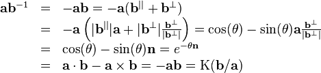
which is the inverse of , as expected, that rotates by  round the same axis .
The product ab
The product gives
![\begin{array}{rcl}
\mathbf{a}\mathbf{b} & = & \mathbf{a}\mathbf{b}^{-1} \mathbf{b}^{2}
=-\mathbf{a}\mathbf{b}^{-1}\\
& = & e^{\pi \mathbf{n}} e^{- \theta \mathbf{n}} =e^{( \pi - \theta )
\mathbf{n}}\\
& = & - \left[ \mathrm{cos} ( - \theta ) + \sin ( - \theta )
\mathbf{n} \right] =- \mathrm{cos} ( \theta ) + \sin ( \theta )
\mathbf{n}\\
& = & -\mathbf{a} \cdot \mathbf{b}+\mathbf{a} \times \mathbf{b}= \mathrm{K}
( \mathbf{b}\mathbf{a} )\end{array}](../I/m/d73d7ccab984000a5bfaef52c6f3787a.png)
showing that, compared to the quotient , the product rotates by the supplement angle round the same axis .
Pairs of conjugate versors
Notice that  &
&  , and
, and  &
&  are two pairs of conjugate versors. Conjugates have the same angle of rotation but round inverse axes, and therefore rotate in opposite directions. The conjugate of a versor is also its inverse, so they are both pairs of inverses.
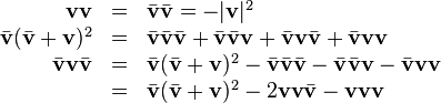
The rotation formula (b/a)v(a/b)
For the -plane of the biradial , the unit vectors and span the plane and are a basis for vectors in the plane so that any vector in the plane can be written in the form  . The unit vector spans the 3rd linearly independent spatial dimension. An arbitrary vector of the pure quaternion vector space can be written
  , where
  is the component in the -plane and
  is the component perpendicular to the -plane.
The biradial applied to an arbitrary vector gives
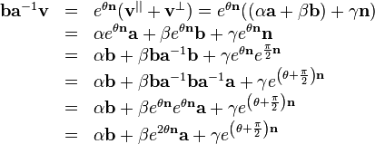
where 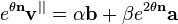 is the component of in the -plane and rotated by in the plane. The other value
  is another quaternion that rotates by
  and scales by
  , and by itself it is not a useful part of the result; this quaternion value can be eliminated as follows
where we recognize 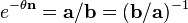 . This suggests trying the following
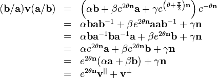
and finding that, in general,  rotates the component of in the plane of the biradial by twice the angle of the biradial, and it leaves the component of perpendicular to the plane unaffected. This type of rotation is called conical rotation due to how the line turns on a cone as it is rotated through an entire round as the axis of the cone.
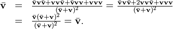
The rays a,b of biradial b/a need not be unit vectors
Although and were treated as unit vectors for simplicity, the result

shows that and need not be unit vectors. Since the lengths of and are inconsequential in the rotation, they are sometimes called rays of the biradial instead of vectors, as mentioned at the beginning.
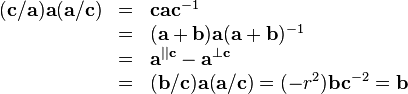
The conical rotation by pi, reflection, or conjugation ba/b
In the work above, we encountered 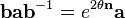 as a planar rotation; this can also be viewed as a conical rotation by
  round as the cone axis, or viewed as a reflection of in
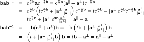
This result  is also called the conjugation of by .
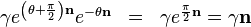
For quadrantal versor (unit vector) perpendicular to vector ,

which is the conjugation of or  , and it is also called the inversion of .
Rotations as successive reflections in vectors
The conical rotation  of by in the plane of the biradial with angle can also be seen as two successive reflections
where  is the first reflection of in , and
  is the second reflection of in .
Equivalent versors
Every pair of unit vectors  in the same plane and having the same angle from
  to
to  form the same biradial
  with same angle
  and same normal
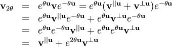
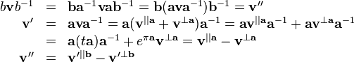
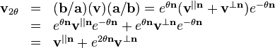
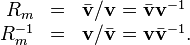
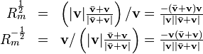
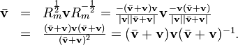
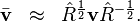
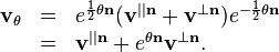
The square root of a versor
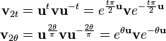
Since rotates by , if we want to rotate by just then we need to take the square root of as
resulting in the formula for rotation by in the plane normal to unit vector
![\begin{array}{rcl}
\mathbf{v}_{\theta} & = & e^{\frac{\theta}{2} \mathbf{n}} \mathbf{v}e^{-
\frac{\theta}{2} \mathbf{n}}\\
& = & \left[ \mathrm{cos} \left( \frac{\theta}{2} \right) + \sin
\left( \frac{\theta}{2} \right) \mathbf{n} \right] \mathbf{v} \left[
\mathrm{cos} \left( \frac{\theta}{2} \right) - \sin \left(
\frac{\theta}{2} \right) \mathbf{n} \right] .\end{array}](../I/m/10e1f2ca75bbdcc60a7c843f588ff423.png)
In theorems it is proved that any quaternion rotation can be expressed as  successive reflections in vectors that reduces to a single conical rotation round a single resultant versor axis by a certain angle , which may be expressed as the versor operator
 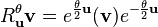 .
.
To apply a rotation by in steps, use the  th-root of , and its conjugate, successively times
If  , then the versor
  can also be written as
and the rotation of vector by in the -plane, or round its normal , can be written as
so that the rotation is seen as various reflections. For example, if  , then
and this rotation is the reflection of in  .
.
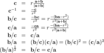
If , then the sum  is the diagonal vector that bisects the rhombus parallelogram framed by and and is the reflector of into or into .
Rodrigues rotation formula and identity to quaternion rotation formula
Another formula for rotation can be derived without quaternions, using only vector analysis which includes vector addition and subtraction and the vector dot and cross products. The formula is known as the Rodrigues Rotation Formula

which rotates any vector conically round the unit vector axis by the angle radians counter-clockwise on right-handed axes or clockwise on left-handed axes according to the matching right-hand or left-hand rule.
This Rodrigues formula is a known result that can be derived without too much difficulty by modeling the problem in vector analysis and finding the solution for  . This formula can also be found from the quaternion rotation formula derived already in terms of biradials
The identity of the quaternion rotation formula to the Rodrigues rotation formula is
where again the unit vector is the axis of conical rotation of vector by according to the handedness described above.
Rotation round arbitrary lines and points
By proper choice of the rotation axis and the angle , the conical rotation  can rotate to any location on the sphere having center
  and radius
  . These conical rotations of occur in circles located on the surface of the sphere, which we can call the sphere of .
There are two types of these circles. A small circle has a radius  , and a great circle has radius
  . If is perpendicular to , the circle of rotation on the sphere is a great circle, and otherwise a small circle. The interior plane of a circle is the base of a rotational cone, with tip or apex at the origin
  . As is rotated, the line of moves on the sides of the cone, and points to different points on the circle at the cone base.
The line  of the rotation axis intersects and intersects the centers of a group of parallel circles in space that section the sphere of by cuts perpendicular to . The line of also intersects the sphere of at the two points called the poles of the rotation where the small circles vanish or degenerate into the poles. The great circle, on the sphere of cut perpendicular to through the center of the sphere of (always the origin of a rotation ), contains the points called the polars of the rotation .
When is one of the two poles (a pole vector) of the rotation , then is parallel to and it rotates in the point (degenerated circle) of the pole and is unaffected by the rotation . When is a polar (a polar vector) of the rotation , then is perpendicular to and is rotated in the great circle of the sphere of perpendicular to , polar to pole  . Otherwise, the rotation of can be viewed in terms of its components parallel and perpendicular to the axis as a cylindrical rotation
where  is polar of the rotation
  (planar rotation) and
  is a pole of the rotation
  (null rotation). The component is rotated in the base of the cylinder in the plane perpendicular to intersecting the origin of the rotation, and the component
  is the translation up the side of the cylinder to the small circle on the sphere of . The vector component is also called an eigenvector (“eigen” is German for “own”) of the rotation . The sum
  is still rotated on a cone inside the cylinder and is a conical rotation of round .
The quadrantal versor, unit vector, could also be called an axial vector or a pole vector of a rotation on the sphere of , the unit sphere. All vectors  perpendicular to the axial vector could be called planar-polar vectors relative to all vectors
  parallel to which could be called axial-pole vectors, where could also be called the unit axial-pole vector. Any circle round axis , in a plane perpendicular to and centered on the line of , could be called a polar circle of . The rotation
  of a planar-polar vector of the rotation is a planar rotation

and the rotation  of an axial-pole vector (eigenvector) of the rotation is a null rotation
The pole round which counter-clockwise rotation is seen by right-hand rule on right-handed axes (holding the pole vector in right-hand) can be called the north geometric pole of the rotation, and the inverse pole called the south geometric pole of the rotation where left-hand rule on left-handed axes would see clockwise rotation (holding the inverse pole vector in left-hand as if it were the positive direction of the axis). A pole, as a point on the sphere, or as a vector from the sphere center to the pole, are synonymous for the purpose considered here, but they can be made as distinct mathematical values in the more advanced Clifford geometric algebras of generalized projective geometry. With this terminology, the quadrantal versor is a unit axial-pole vector of the unit sphere of (the unit sphere) and is directed toward the point of the north geometric pole of the rotation on right-handed axes, or directed toward the south geometric pole on left-handed axes where positive rotations are then taken clockwise. This convention or orientation of north and south geometric poles matches the geometric poles and rotation of the Earth.
If the sphere of relative to an origin is considered the set

of vectors  , then
  can be considered the rotation of the entire sphere. This notation is meant to convey that subtraction by , followed by application of rotation
  , followed by addition of is to occur on each element of the set
  of vectors that are located on the surface of the sphere defined by and by the invariant radial distance
  that any other point on the sphere surface must also have.
The rotations  are limited to rotating spheres of radius , with surface points
  , and that are concentric spheres centered on the origin
  of space.
The rotation of spheres concentric on any arbitrary origin  is the rotation
  . The spheres are centered at
  , and determines a particular radius
  .
.
The rotation of an entire sphere, as a set of vector elements , shows that translation (to and from) relative to the sphere origin is generally required for rotation of vectors round the surface of an arbitrary sphere located in space.
The usual concern is not rotating entire spheres, but is rotating a particular point perpendicularly round an arbitrary line that does not necessarily intersect the origin  , or is to rotate round an arbitrary point .
An arbitrary line can be represented by  . We want to rotate round this line as the rotational axis. The rotation will occur in a circle in space, and this circle is on the sphere centered at with radius , and the rotational axis is parallel to the unit vector . The center of the circle is at
 ![\mathbf{c}=\mathcal{P}_{\mathbf{n}} ( \mathbf{v}-\mathbf{o}' ) +\mathbf{o}' = [ ( \mathbf{v}-\mathbf{o}' ) \cdot \mathbf{n} ] \mathbf{n}+\mathbf{o}'](../I/m/e1dd229ed9356f01d6ad045691e5f6e1.png) . The location of relative to the circle center is
. The location of relative to the circle center is  .
.
The rotation of round the line is
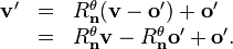
If we viewed as an arbitrary point that we wished to rotate round, then we still needed to specify a rotational axis through , and the rotation is
![\begin{array}{rcl}
\mathbf{v}' & = & R^{\theta}_{\mathbf{n}} ( \mathbf{v}-\mathbf{c} )
+\mathbf{c}\\
& = & R^{\theta}_{\mathbf{n}} [ \mathbf{v}-\mathcal{P}_{\mathbf{n}} (
\mathbf{v}-\mathbf{o}' ) -\mathbf{o}' ] +\mathbf{c}\\
& = & R^{\theta}_{\mathbf{n}} \mathbf{v}-R^{\theta}_{\mathbf{n}}
\mathcal{P}_{\mathbf{n}} ( \mathbf{v}-\mathbf{o}' ) -R^{\theta}_{\mathbf{n}}
\mathbf{o}' +\mathbf{c}\\
& = & R^{\theta}_{\mathbf{n}} \mathbf{v}-\mathcal{P}_{\mathbf{n}} (
\mathbf{v}-\mathbf{o}' ) -R^{\theta}_{\mathbf{n}} \mathbf{o}' +\mathbf{c}\\
& = & R^{\theta}_{\mathbf{n}} \mathbf{v}- ( \mathbf{c}-\mathbf{o}' )
-R^{\theta}_{\mathbf{n}} \mathbf{o}' +\mathbf{c}\\
& = & R^{\theta}_{\mathbf{n}} \mathbf{v}-R^{\theta}_{\mathbf{n}}
\mathbf{o}' +\mathbf{o}' .\end{array}](../I/m/37216b991411bd17addb47321eb58241.png)
Vector-arcs
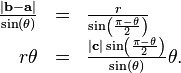
A vector-arc can be represented by the vector chord  in the circle where is rotated to by a quaternion biradial through an arc
  of the circle that can be given by law of sines as
The rotation can also be seen as the translation of by vector-arc across the chord  . The operation to can be written multiplicatively or additively
as quaternion multiplication or vector-arc addition.
The vector-arc  can be added to another different vector
  as
as  , where
  is viewed as being
  rotated in the same relative direction
  and by the same arc on a sphere centered at a same relative position as to and . The vector-arcs, or chords, of the rotations
 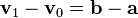 correspond. Some successive rotations applied to produces successive vector-arcs
 . The vector-arcs can be added successively to vector as
  and each one of these vectors remains on a sphere or path corresponding to the sphere or path of .
Since the order, or sequence, of adding vector-arcs onto (adding successively) is important for replaying a sequence of vector-arc translations on a sphere or path, when a vector-arc is added to  , the next vector-arc
  added to
  is a specific vector-arc representing the next rotation and is called the provector-arc of the prior vector-arc . The sum of a vector-arc and its provector-arc is their transvector-arc
  representing an arcual sum[1](Art.218).
The addition of vector-arcs equals successive rotations in the same sphere only if the vector-arcs are successive corresponding chords in the same sphere. The successive chords form a gauche[1](Art.323) or skew polygon inscribed in the sphere. To remain on the same sphere, the addition of the vector-arcs to must be in rotations order, translating across a specific sequence of chords representing the rotation arcs and sides of a gauche polygon inscribed in the sphere. As chords are added to in rotations sequence, the resulting positions of vertices of the polygon in the sphere are found. The effect is to replay a specific sequence of translations starting at , with vector-arcs added head to tail as the polygon sides or chords in the sphere. Direct rotations among the found points of the inscribed polygon can be computed as other transvector-arcs.
A sequence of vector-arcs can be pre-generated and applied in sequence forward (adding the provector-arc) and backward (subtracting the prior provector-arc). The sequences of vector-arcs could be applied to multiple points using additions or their pre-additions (transvector-arcs), which may be much faster than multiplying each point using a quaternion operator.
Mean versor
The mean versor problem can be described as follows: If given versors
where each versor rotates by the angle  in the plane perpendicular to the unit vector
  , then the vector can be rotated into different points using the half-angle (or full-angle) versors
For  , the three vectors
  are the vertices of a spherical triangle
  . The location of the spherical centroid
  of represents the true mean rotation of relative to the three vertices.
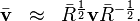
As a first approach to trying to find and the mean versor  , we can consider the average of the vectors , scaled to touch the sphere, as approximately . With this approach, the spherical centroid of is approximately
on the condition that the vertices are clustered closely together such that the angle between any two vertices does not exceed  radians. For any , this condition is satisfied if

when using the half-angle versors, or if

when using the full-angle versors.
Under this condition, this formula for the spherical centroid of has good accuracy. For angles exceeding these conditions, the error increases rapidly up to the error extremum or worse-possible error when two vertices reach radians apart!
For  , the vector is generally not the centroid of a spherical polygon of the vertices , but does approximate the true mean rotation of .
The approximate mean versor is
The approximate mean versor with half the angle is
The rotation of by the approximate mean versor  is
is
Using the identities
we can verify that
By this first approach, this approximate mean versor is dependent on a particular and adapts well to a wide range versors  . It is computationally expensive since it requires computing all the rotations and averaging them. A potential problem of this approach is the possibly unacceptable error when two different are very close to radians apart, or are nearly inversions.
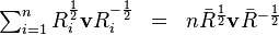
As a second approach to trying to find and the mean versor , we can consider using the average vector-arc of the vector-arcs  represented by the versors . By this approach, we try the geometric mean of the versors
![\begin{array}{rcl}
\hat{R} & = & \sqrt[n]{\prod_{i = 1}^n R_i}\\
& = & e^{(\theta_1 \mathbf{r}_1 + \theta_2 \mathbf{r}_2 + \cdots + \theta_n
\mathbf{r}_n) / n}\end{array}](../I/m/742275e179d3c84910cadcffeb48df6b.png)
as approximating the true mean versor. Each can be interpreted as a vector-arc, and

as the average vector-arc.
By this method, the approximate mean rotation of is
Good accuracy is achieved using the same condition  as in the first approach.
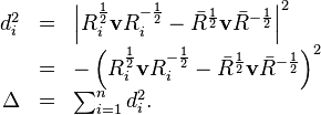
As a third approach to trying to find and the mean versor , the solution is to find the versor  that minimizes the distance
  , where
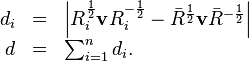
We can also choose to minimize the sum of squares
We can write  as
as
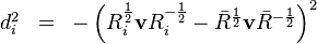
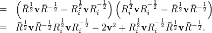
Now we can write  as
as

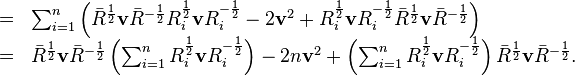
If
then  and is minimized. This can be expanded as

which shows more clearly that the closer is to each , then the closer is to zero. This minimization is achieved by the arithmetic mean
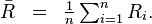
This result does not depend on a particular . Technically, a versor should always have unit magnitude, but generally  . The quaternion can be normalized to have unit magnitude if necessary, but when used in the following versor rotation operation, any magnitude of cancels anyway.
By this approach, the approximate mean rotation of is
Once again, good accuracy is achieved using the same condition as in the first and second approaches.
Each approach has a different behavior as angles are increased. For , they give nearly identical results. Each approach may be worth comparing to the others for a particular problem.
Testing the approaches: One way to experiment interactively with these formulas is to use the program GAViewer and have it open and run the following file mean-versor.g:
/* mean-versor.g Mean Versor Demo */
// Use ctrl-rightmousebutton to drag vectors v r1 r2 r3
// around the sphere and see rotations change dynamically.
// Sliders for angles t1 t2 t3 also trigger dynamic changes.

// Lines ending with , ARE rendered
// Lines ending with ; ARE NOT rendered

// Reset the viewer.
reset();
set_window_title("Mean Versor Demo");

// Run a .geo format command.
// Certain things can only be done with geo commands.
// Set the text parsing/formatting mode for the text of labels.
cmd("tsmode equation");
// Equation mode formats text like Latex equation mode does.

// Draw basic x,y,z direction unit vectors.
x=e1,
y=e2,
z=e3,
label(x),
label(y),
label(z),

// Pseudoscalar I.
// Needed to compute duals; i.e,
// to convert vectors to pure quaternions in geometric algebra.
I = e1 e2 e3;
// Draw a unit ball or sphere.
B = 4/3 pi pow(0.80,2) e1 e2 e3;
B = color(B,1,1,1,0.25),

// Initial point v on unit radius sphere.
// This is the vector we are rotating.
v = (e1+e2+e3);
v = v / norm(v);
label(v),

// Make angles t1,t2,t3 in degrees here
// but converted to radians in formulas later.
ctrl_range(t1= 40,-180,180);
ctrl_range(t2=-25,-180,180);
ctrl_range(t3=-15,-180,180);
// Use half-angle versor rotation formulas below.

// Make versors R1 R2 R3 that rotate round axes r1 r2 r3
// that are initially close to e1 e2 e3 (but can be dragged).
r1 = (5 e1 +   e2 +   e3);
r2 = (  e1 + 5 e2 +   e3);
r3 = (  e1 +   e2 + 5 e3);
r1 = r1 / norm(r1),
r2 = r2 / norm(r2),
r3 = r3 / norm(r3),
label(r1),
label(r2),
label(r3),
R1 = exp( t1/2 pi/180 r1/I );
R2 = exp( t2/2 pi/180 r2/I );
R3 = exp( t3/2 pi/180 r3/I );

// Rotate v into v1 v2 v3 using R1 R2 R3.
v1 = R1 v / R1,
v2 = R2 v / R2,
v3 = R3 v / R3,
label(v1),
label(v2),
label(v3),

// Locate the mean rotation of v directly from the mean of v1 v2 v3.
// This is the accurate approximation of the centroid or mean rotation of v.
// This is dependent on a particular v and on the versors R1 R2 R3.
m = (v1+v2+v3)/norm(v1+v2+v3),
label(m),

// Locate the mean rotation of v using the geometric mean of R1 R2 R3
// which is thought of as using the mean vector-arc.
G = exp( ((t1/2 pi/180 r1)+(t2/2 pi/180 r2)+(t3/2 pi/180 r3))/(3I) );
g = G v / G,
label(g),

// Locate the mean rotation of v using the arithmetic mean of R1 R2 R3
// normalized to unit norm for a proper versor.
A = (R1+R2+R3)/norm(R1+R2+R3);
a = A v / A,
label(a),

// Begin dynamic element.
// Simply recalculate everything in here.
dynamic{d1:

// The basis should not be moved.
x=e1,
y=e2,
z=e3,
x= color(x,0,0,0,0.5),
y= color(y,0,0,0,0.5),
z= color(z,0,0,0,0.5),

// The sphere.
B = 4/3 pi pow(0.80,2) e1 e2 e3;
B = color(B,1,1,1,0.25),

// The vector we are rotating around a unit radius sphere.
v = v / norm(v),

// Make versors R1 R2 R3 that rotate round axes r1 r2 r3
// and that are initially set close to e1 e2 e3.
r1 = r1 / norm(r1),
r2 = r2 / norm(r2),
r3 = r3 / norm(r3),
r1 = color(r1,1,1,0,0.5),
r2 = color(r2,1,1,0,0.5),
r3 = color(r3,1,1,0,0.5),
R1 = exp( t1/2 pi/180 r1/I );
R2 = exp( t2/2 pi/180 r2/I );
R3 = exp( t3/2 pi/180 r3/I );

// Rotate v into v1 v2 v3 using R1 R2 R3.
v1 = R1 v / R1,
v2 = R2 v / R2,
v3 = R3 v / R3,
v1 = color(v1,0,0,1,0.5),
v2 = color(v2,0,0,1,0.5),
v3 = color(v3,0,0,1,0.5),

// Locate the mean rotation of v directly from the mean of v1 v2 v3.
m = norm(v) (v1+v2+v3)/norm(v1+v2+v3),
m = color(m,1,0,1,0.5),

// Locate the mean rotation of v using the geometric mean of R1 R2 R3.
G = exp( ((t1/2 pi/180 r1)+(t2/2 pi/180 r2)+(t3/2 pi/180 r3))/(3I) );
g = G v / G,
g = color(g,1,0,1,0.5),

// Locate the mean rotation of v using the arithmetic mean of R1 R2 R3.
// The magnitude of A does not matter here.
A = (R1+R2+R3);
a = A v / A,
a = color(a,1,0,1,0.5),
}
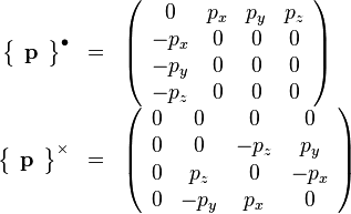
Matrix representations of quaternions and rotations
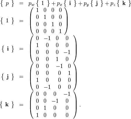
A quaternion can be written as a  -tuple of scalar components or as a -element column vector, and it can also be written as a
  matrix by expanding the quaternion product
![\begin{array}{rcl}
\left[ \begin{array}{l}
p q
\end{array} \right] & = & \left(\begin{array}{c}
p_{w} q_{w} -p_{x} q_{x} -p_{y} q_{y} -p_{z} q_{z}\\
p_{x} q_{w} +p_{w} q_{x} -p_{z} q_{y} +p_{y} q_{z}\\
p_{y} q_{w} +p_{z} q_{x} +p_{w} q_{y} -p_{x} q_{z}\\
p_{z} q_{w} -p_{y} q_{x} +p_{x} q_{y} +p_{w} q_{z}
\end{array}\right)\\
\left\{ \begin{array}{l}
p
\end{array} \right\} \left[ \begin{array}{l}
q
\end{array} \right] & = & \left(\begin{array}{cccc}
p_{w} & -p_{x} & -p_{y} & -p_{z}\\
p_{x} & p_{w} & -p_{z} & p_{y}\\
p_{y} & p_{z} & p_{w} & -p_{x}\\
p_{z} & -p_{y} & p_{x} & p_{w}
\end{array}\right) \left(\begin{array}{c}
q_{w}\\
q_{x}\\
q_{y}\\
q_{z}
\end{array}\right)\end{array}](../I/m/1cb16f2a9339b9f535f81bf024b5e199.png)
and factoring the resulting column vector form ![\left[ \begin{array}{l} p q \end{array} \right]](../I/m/2442c77aab9bcc4cdf8fa074ef072bb0.png) into a matrix-vector product
into a matrix-vector product ![\left\{ \begin{array}{l} p \end{array} \right\} \left[ \begin{array}{l} q \end{array} \right]](../I/m/bef3033f88615ed8a14bb90ac52e7f40.png) .
.
Quaternions in the matrix form  can be added as
 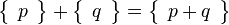 , and can be multiplied together using non-commutative matrix multiplication giving products of the form
 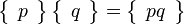 . Quaternions in column vector form
 ![\left[ \begin{array}{l} q \end{array} \right]](../I/m/27127fc8583bd3b1b6b424a3ba9e609e.png) can be added, and can be the multiplicand of a quaternion multiplier in matrix form , giving products
can be added, and can be the multiplicand of a quaternion multiplier in matrix form , giving products ![\left\{ \begin{array}{l} p \end{array} \right\} \left[ \begin{array}{l} q \end{array} \right] = \left[ \begin{array}{l} p q \end{array} \right]](../I/m/13f00960cc3452309e5e895efa09de83.png) in column vector form.
in column vector form.
For two vectors, their product is
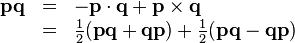
and their matrix-vector product is
![\begin{array}{rcl}
\left\{ \begin{array}{l}
\mathbf{p}
\end{array} \right\} \left[ \begin{array}{l}
\mathbf{q}
\end{array} \right] & = & \left(\begin{array}{cccc}
0 & -p_{x} & -p_{y} & -p_{z}\\
p_{x} & 0 & -p_{z} & p_{y}\\
p_{y} & p_{z} & 0 & -p_{x}\\
p_{z} & -p_{y} & p_{x} & 0
\end{array}\right) \left(\begin{array}{c}
0\\
q_{x}\\
q_{y}\\
q_{z}
\end{array}\right)\\
& = & \left(\begin{array}{c}
-p_{x} q_{x} -p_{y} q_{y} -p_{z} q_{z}\\
-p_{z} q_{y} +p_{y} q_{z}\\
p_{z} q_{x} -p_{x} q_{z}\\
-p_{y} q_{x} +p_{x} q_{y}
\end{array}\right) = \left(\begin{array}{c}
- ( \mathbf{p} \cdot \mathbf{q} )\\
\left[ \begin{array}{l}
\mathbf{p} \times \mathbf{q}
\end{array} \right]_{x}\\
\left[ \begin{array}{l}
\mathbf{p} \times \mathbf{q}
\end{array} \right]_{y}\\
\left[ \begin{array}{l}
\mathbf{p} \times \mathbf{q}
\end{array} \right]_{z}
\end{array}\right)\end{array}](../I/m/bee2eea65c33ed7ad343696ffe57fc2f.png)
![\begin{array}{rcl}
\left\{ \begin{array}{l}
\mathbf{p}
\end{array} \right\} & = & - \left\{ \begin{array}{l}
\mathbf{p}
\end{array} \right\}^{\bullet} + \left\{ \begin{array}{l}
\mathbf{p}
\end{array} \right\}^{\times}\\
\left[ \begin{array}{l}
\mathbf{p} \cdot \mathbf{q}
\end{array} \right] & = & \left\{ \begin{array}{l}
\mathbf{p}
\end{array} \right\}^{\bullet} \left[ \begin{array}{l}
\mathbf{q}
\end{array} \right]\\
\left[ \begin{array}{l}
\mathbf{p} \times \mathbf{q}
\end{array} \right] & = & \left\{ \begin{array}{l}
\mathbf{p}
\end{array} \right\}^{\times} \left[ \begin{array}{l}
\mathbf{q}
\end{array} \right]\\
\left[ \begin{array}{l}
\mathbf{p}\mathbf{q}
\end{array} \right] & = & \left( - \left\{ \begin{array}{l}
\mathbf{p}
\end{array} \right\}^{\bullet} + \left\{ \begin{array}{l}
\mathbf{p}
\end{array} \right\}^{\times} \right) \left[ \begin{array}{l}
\mathbf{q}
\end{array} \right] =- \left[ \begin{array}{l}
\mathbf{p} \cdot \mathbf{q}
\end{array} \right] + \left[ \begin{array}{l}
\mathbf{p} \times \mathbf{q}
\end{array} \right]\end{array}](../I/m/cdfa7b301d38847ff5e7fb5842ccee13.png)
which gives matrices representing dot and cross product operators on column vectors.
The dot and cross products for two vectors in matrix forms are
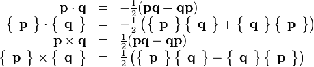
which take the symmetric and anti-symmetric parts of the vector product  .
.
The matrix form can be decomposed into a sum of matrices to identify the matrix representations of as
A quaternion rotation, by radians, of vector round the unit vector axis can be written as
To write this rotation in matrix-vector multiplication form, we first need some more identities.
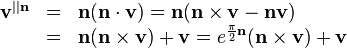
The vector component of parallel to the unit vector is
![\begin{array}{rcl}
\left[ \begin{array}{l}
\mathbf{v}^{||\mathbf{n}}
\end{array} \right] & = & \left[ \begin{array}{l}
\mathbf{n}
\end{array} \right] \left[ \begin{array}{l}
\mathbf{n}
\end{array} \right]^{\mathrm{T}} \left[ \begin{array}{l}
\mathbf{v}
\end{array} \right]\end{array}](../I/m/1fb91f7d317517f1bd27d232214b2ddc.png)
![\begin{array}{rcl}
& = & \left(\begin{array}{c}
0\\
n_{x}\\
n_{y}\\
n_{z}
\end{array}\right) \left(\begin{array}{cccc}
0 & n_{x} & n_{y} & n_{z}
\end{array}\right) \left(\begin{array}{c}
0\\
v_{x}\\
v_{y}\\
v_{z}
\end{array}\right)\\
& = & \left\{ \begin{array}{l}
\mathbf{n}
\end{array} \right\} \left\{ \begin{array}{l}
\mathbf{n}
\end{array} \right\}^{\times} \left[ \begin{array}{l}
\mathbf{v}
\end{array} \right] + \left[ \begin{array}{l}
\mathbf{v}
\end{array} \right] = \left( \left\{ \begin{array}{l}
\mathbf{n}
\end{array} \right\} \left\{ \begin{array}{l}
\mathbf{n}
\end{array} \right\}^{\times} + \left\{ \begin{array}{l}
1
\end{array} \right\} \right) \left[ \begin{array}{l}
\mathbf{v}
\end{array} \right]\\
& = & \left\{ \begin{array}{l}
\mathbf{n}
\end{array} \right\} \left\{ \begin{array}{l}
\mathbf{n}
\end{array} \right\}^{\bullet} \left[ \begin{array}{l}
\mathbf{v}
\end{array} \right]\\
& = & \left\{ \begin{array}{l}
\mathbf{n}
\end{array} \right\}^{||} \left[ \begin{array}{l}
\mathbf{v}
\end{array} \right] = \left(\begin{array}{cccc}
1 & 0 & 0 & 0\\
0 & n_{x} n_{x} & n_{x} n_{y} & n_{x} n_{z}\\
0 & n_{y} n_{x} & n_{y} n_{y} & n_{y} n_{z}\\
0 & n_{z} n_{x} & n_{z} n_{y} & n_{z} n_{z}
\end{array}\right) \left(\begin{array}{c}
0\\
v_{x}\\
v_{y}\\
v_{z}
\end{array}\right)\end{array}](../I/m/22b05c4eabcb0956eeaa1382b122721e.png)
The vector component of perpendicular to the unit vector is

![\begin{array}{rcl}
\left[ \begin{array}{l}
\mathbf{v}^{\bot \mathbf{n}}
\end{array} \right] & = & \left[ \begin{array}{l}
\mathbf{v}
\end{array} \right] - \left[ \begin{array}{l}
\mathbf{v}^{||\mathbf{n}}
\end{array} \right] = \left[ \begin{array}{l}
\mathbf{v}
\end{array} \right] - \left\{ \begin{array}{l}
\mathbf{n}
\end{array} \right\}^{||} \left[ \begin{array}{l}
\mathbf{v}
\end{array} \right]\end{array}](../I/m/1e8a722db249ad6ae987604991ccf6db.png)
![\begin{array}{rcl}
& = & \left( \left\{ \begin{array}{l}
1
\end{array} \right\} - \left\{ \begin{array}{l}
\mathbf{n}
\end{array} \right\}^{||} \right) \left[ \begin{array}{l}
\mathbf{v}
\end{array} \right]\\
& = & \left\{ \begin{array}{l}
\mathbf{n}
\end{array} \right\}^{\bot} \left[ \begin{array}{l}
\mathbf{v}
\end{array} \right] = \left(\begin{array}{cccc}
0 & 0 & 0 & 0\\
0 & 1-n_{x} n_{x} & -n_{x} n_{y} & -n_{x} n_{z}\\
0 & -n_{y} n_{x} & 1-n_{y} n_{y} & -n_{y} n_{z}\\
0 & -n_{z} n_{x} & -n_{z} n_{y} & 1-n_{z} n_{z}
\end{array}\right) \left(\begin{array}{c}
0\\
v_{x}\\
v_{y}\\
v_{z}
\end{array}\right)\\
& = & - \left\{ \begin{array}{l}
\mathbf{n}
\end{array} \right\} \left\{ \begin{array}{l}
\mathbf{n}
\end{array} \right\}^{\times} \left[ \begin{array}{l}
\mathbf{v}
\end{array} \right] .\end{array}](../I/m/acc398a39549ea740dd6e859f8c2a6d4.png)
The rotor  for the rotation round axis by angle is
The rotation can also be written
which appears to be a smaller form of the Rodrigues rotation formula. Starting here, we have enough identities to switch into matrices and column vectors as
![\begin{array}{rcl}
\left[ \begin{array}{l}
\mathbf{v}_{\theta}
\end{array} \right] & = & \left\{ \begin{array}{l}
\mathbf{n}
\end{array} \right\}^{||} \left[ \begin{array}{l}
\mathbf{v}
\end{array} \right] + \left\{ \begin{array}{l}
e^{\theta \mathbf{n}}
\end{array} \right\} \left\{ \begin{array}{l}
\mathbf{n}
\end{array} \right\}^{\bot} \left[ \begin{array}{l}
\mathbf{v}
\end{array} \right]\\
& = & \left( \left\{ \begin{array}{l}
\mathbf{n}
\end{array} \right\}^{||} + \left\{ \begin{array}{l}
e^{\theta \mathbf{n}}
\end{array} \right\} \left\{ \begin{array}{l}
\mathbf{n}
\end{array} \right\}^{\bot} \right) \left[ \begin{array}{l}
\mathbf{v}
\end{array} \right]\\
& = & \left( \left\{ \begin{array}{l}
\mathbf{n}
\end{array} \right\}^{||} + \left( \left\{ \begin{array}{l}
c
\end{array} \right\} +s \left\{ \begin{array}{l}
\mathbf{n}
\end{array} \right\} \right) \left( - \left\{ \begin{array}{l}
\mathbf{n}
\end{array} \right\} \left\{ \begin{array}{l}
\mathbf{n}
\end{array} \right\}^{\times} \right) \right) \left[ \begin{array}{l}
\mathbf{v}
\end{array} \right]\\
& = & \left( \left\{ \begin{array}{l}
\mathbf{n}
\end{array} \right\}^{||} -c \left\{ \begin{array}{l}
\mathbf{n}
\end{array} \right\} \left\{ \begin{array}{l}
\mathbf{n}
\end{array} \right\}^{\times} +s \left\{ \begin{array}{l}
\mathbf{n}
\end{array} \right\}^{\times} \right) \left[ \begin{array}{l}
\mathbf{v}
\end{array} \right]\\
& = & \left( \left\{ \begin{array}{l}
\mathbf{n}
\end{array} \right\}^{||} +c \left( \left\{ \begin{array}{l}
1
\end{array} \right\} - \left\{ \begin{array}{l}
\mathbf{n}
\end{array} \right\}^{||} \right) +s \left\{ \begin{array}{l}
\mathbf{n}
\end{array} \right\}^{\times} \right) \left[ \begin{array}{l}
\mathbf{v}
\end{array} \right]\\
& = & \left( \left\{ \begin{array}{l}
\mathbf{n}
\end{array} \right\}^{||} + \left\{ \begin{array}{l}
c
\end{array} \right\} -c \left\{ \begin{array}{l}
\mathbf{n}
\end{array} \right\}^{||} +s \left\{ \begin{array}{l}
\mathbf{n}
\end{array} \right\}^{\times} \right) \left[ \begin{array}{l}
\mathbf{v}
\end{array} \right]\\
& = & \left( ( 1-c ) \left\{ \begin{array}{l}
\mathbf{n}
\end{array} \right\}^{||} + \left\{ \begin{array}{l}
c
\end{array} \right\} +s \left\{ \begin{array}{l}
\mathbf{n}
\end{array} \right\}^{\times} \right) \left[ \begin{array}{l}
\mathbf{v}
\end{array} \right]\\
& = & \left\{ \begin{array}{l}
R^{\theta}_{\mathbf{n}}
\end{array} \right\} \left[ \begin{array}{l}
\mathbf{v}
\end{array} \right]\end{array}](../I/m/26f1599f2c38a5fb39a67bb48c77690e.png)
which can be written as the matrix-vector product
![\begin{array}{rcl}
\left[ \begin{array}{l}
\mathbf{v}_{\theta}
\end{array} \right] & = & \left\{ \begin{array}{l}
R^{\theta}_{\mathbf{n}}
\end{array} \right\} \left[ \begin{array}{l}
\mathbf{v}
\end{array} \right]\end{array}](../I/m/79c776c321d94691d3aa7ae1138f5298.png)
![\begin{array}{rcl}
& = & \left( \begin{array}{l}
( 1-c ) \left(\begin{array}{cccc}
1 & 0 & 0 & 0\\
0 & n_{x} n_{x} & n_{x} n_{y} & n_{x} n_{z}\\
0 & n_{y} n_{x} & n_{y} n_{y} & n_{y} n_{z}\\
0 & n_{z} n_{x} & n_{z} n_{y} & n_{z} n_{z}
\end{array}\right) +\\
\left(\begin{array}{cccc}
c & 0 & 0 & 0\\
0 & c & 0 & 0\\
0 & 0 & c & 0\\
0 & 0 & 0 & c
\end{array}\right) +s \left(\begin{array}{cccc}
0 & 0 & 0 & 0\\
0 & 0 & -n_{z} & n_{y}\\
0 & n_{z} & 0 & -n_{x}\\
0 & -n_{y} & n_{x} & 0
\end{array}\right)
\end{array} \right) \left[ \begin{array}{l}
\mathbf{v}
\end{array} \right]\\
& = & \left(\begin{array}{cccc}
1 & 0 & 0 & 0\\
0 & ( 1-c ) n_{x} n_{x} +c & ( 1-c ) n_{x} n_{y} -s n_{z} & ( 1-c ) n_{x}
n_{z} +s n_{y}\\
0 & ( 1-c ) n_{y} n_{x} +s n_{z} & ( 1-c ) n_{y} n_{y} +c & ( 1-c ) n_{y}
n_{z} -s n_{x}\\
0 & ( 1-c ) n_{z} n_{x} -s n_{y} & ( 1-c ) n_{z} n_{y} +s n_{x} & ( 1-c )
n_{z} n_{z} +c
\end{array}\right) \left[ \begin{array}{l}
\mathbf{v}
\end{array} \right]\end{array}](../I/m/0c49a7d5d6971acf97ec1d69ade1abdc.png)
where this matrix represents the rotation operator. The lower  part of the matrix is all that is needed to rotate vectors in 3D. The full matrix can be used to rotate quaternions, where any scalar part is unaffected by the rotation and the vector part is rotated in the usual way.
Rotations round the axes are found by setting as one of them, which gives
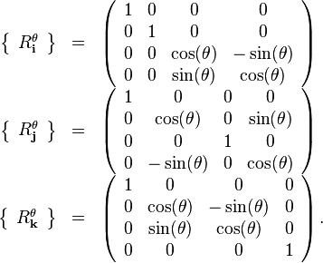
A rotation by a negative angle is the same as a change of basis onto axes rotated by the positive angle. Cramer's rule, and related methods, provide a more generalized way to compute vectors relative to a new or changed basis.
Relationship between quaternions and complex numbers
The relationship between complex numbers and quaternions, with respect to planar rotations by radians in the vector plane perpendicular to , might be written as
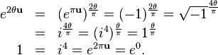
This seems to show that  must be identified with
  representing a planar rotation by or a null rotation round , otherwise the results degenerate. The value (not to be confounded as the quaternion unit
  ) seems to represent rotation by round since
In general,  seems to represent quadrants of rotation round . However, this interpretation of holds for any arbitrary axis , such that can always be interpreted as a versor that is perpendicular to any and all geometrical (generally non-commutative multiplication) planes spanned by arbitrary biradials, or that is parallel and equivalent to all axes of rotation on the unit-sphere.
On a metrical (generally commutative multiplication) complex number plane where points  are represented by complex numbers
  , the value is a quadrantal rotation operator on the points

If is temporarily identified with (as an isomorphism), then  can be interpreted simultaneously as both a geometrical rotation operator on geometrical vectors in the -plane and as a metrical rotation operator on metrical points represented by complex numbers
  .
.
In standard quaternions, the scalars  are limited to real numbers so that complex numbers
  are not elements of the set of standard quaternion numbers. This means that using within standard or real quaternions is not permitted. Therefore, the identification of with , or trying
  is not valid. In the above, the words “might” and “seems” are emphasized because
  , or any power of , is not a valid value to construct within standard quaternions. Stated more clearly, the power

is generally a complex number, and therefore it is not generally permitted in real quaternions.
Whenever a value similar to  is needed, a specific versor having specific geometrical significance on the unit-sphere must be used as a metrical rotation operator on the
  -plane of pseudo-complex numbers
  .
.
In practice, an exception can be made for  and allow this power if is an integer, since the result remains a real number. Expressions of the form are often used to give the sign or orientation of certain results. In general, this exception can cause problems because it is an operation outside of the proper algebra of quaternions.
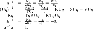
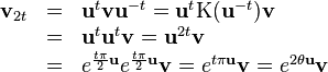
Consider the general case of taking the power of a quaternion
![\begin{array}{rcl}
\mathbf{u} & = & \mathrm{UVU} q= \mathrm{UV} \left( \frac{q}{\mathrm{T} q}
\right) = \mathrm{U} \left( \frac{\mathbf{q}}{\mathrm{T} q} \right) =
\frac{\mathrm{T} q}{\mathrm{T} \mathbf{q}} \mathbf{q}\\
0 \leq \theta & = & \mathrm{cos}^{-1} \left( \mathrm{SU} q \right) =
\mathrm{cos}^{-1} \left( \frac{q_{w}}{\mathrm{T} q} \right) \leq \pi\\
q^{t} & = & \left( \mathrm{T} q \mathrm{U} q \right)^{t} = \left( \mathrm{T}
q \right)^{t} e^{t \theta \mathbf{u}} = \left( \mathrm{T} q \right)^{t}
\left[ \mathrm{cos} ( t \theta ) + \sin ( t \theta ) \mathbf{u}
\right]\end{array}](../I/m/b81792900e5c4ea071951aeeaab9c04e.png)
and notice that tensors are positive and the power of a versor should never require taking the power so long as the axis is known.
If  or
or  then
then  and can be lost, which is a problem where it can be said that a scalar
  , or any scalar by itself, is not a quaternion. It is important to not lose the axis of the quaternion or else the quaternion geometric algebra is not closed, or it has exited into the metrical algebra of real or complex numbers if that is acceptable to your application. Whatever the angle of , the versor expression
  should be retained and not allowed to degenerate into a scalar if remaining in the quaternion algebra is important.
It would appear that quaternions do not really extend metrical real or complex numbers, but forms its very own special geometric algebra that is not closed if the axis (the geometric part) of a quaternion is lost. The paper Planar Complex Numbers in Even n Dimensions and the monograph Complex Numbers in n Dimensions, both by Silviu Olariu and published in 2000, present a possible extension of complex numbers that have commutative multiplication. Higher dimensional extensions of complex numbers are also known as hypercomplex numbers.
In geometric algebras, such as quaternions and Clifford geometric algebras, the value  is usually avoided due to its ambiguous or indeterminate geometrical interpretation. It is avoided by limiting scalars to real numbers and using a subalgebra isomorphic to complex numbers when needed. Again, it is also possible to allow the geometric algebra to exit into the metrical real or complex number algebra if that is acceptable. And again, an exception is integer powers that are commonly used in formulas to compute signs or orientation.
The biquaternions[1](Art.669) include as an element of its algebra, but it might be well to also consider using the Clifford geometric algebra  , wherein complex numbers, quaternions, biquaternions, and dual quaternions are all embedded isomorphically as subalgebras.
Quaternion rotation biradials in Clifford geometric algebra
To keep this article somewhat self-contained, this subsection tries to provide an overview or partial introduction to geometric algebra, with many identities and formulas, aimed at helping the reader to more quickly see how quaternion rotations can be used in geometric algebra. See the references and other works on geometric algebra for general introductions to the subject.
Studying the algebra of rotations teaches a lot about the geometric algebra. In geometric algebra, the products and quotients of vectors are also biradials or transition operators, and are very similar to quaternions. In fact, they are quaternions, but in a different form, with different terminology, and in a different, more generalized algebra. The quotient is still the transition operator that takes to as  . The transition of to is a composition of a rotation into the line of followed by a scaling to the length of .
Quaternion vectors are imaginary directed quantities
A real quaternion  has a pure quaternion or quaternion vector part
  and a scalar part
  , where the scalars
  are limited to real numbers. The real quaternions are simply the quaternions commonly used.
The quaternion vector units are used as a basis for representing points and directed quantities in a three-dimensional space. However, the square  of a vector quantity
  in quaternions is
  . In effect, the directed quantity is treated as a pure imaginary quantity, even though its components
  have been limited to real numbers and the quantity should be considered real and have a real positive squared quantity. This is one of the problems with quaternions and is part of the motivation for avoiding quaternion vector quotients and products in ordinary vector calculus or analysis, as introduced in the 1901 book Vector Analysis[2] by E. B. Wilson that is founded upon the lectures of J. W. Gibbs.
Euclidean vectors are real directed quantities
A different orthonormal basis of base vector units  for three-dimensional space can be used instead of . The directed quantity can be rewritten
  on this basis. If we now require that
  , then we also require that
  . The vector can now be called a Euclidean vector, and are the Euclidean vector units of a three-dimensional Euclidean space that may be variously denoted
  or
or  . The scalars are still limited to real numbers.
Clifford geometric algebras
The algebra, variously denoted  or
or  , of the vector units is called the Clifford geometric algebra of Euclidean
  -space, and is also denoted
  . We are only concerned with this particular Clifford geometric algebra in all that follows here. This algebra differs from the quaternion geometric algebra of . However, the quaternion units are isomorphic to the three unit
  -blades
  of this Clifford algebra, allowing quaternion concepts to be used within the subalgebra of these three unit -blades.
Clifford algebras also allow more vector units than three, and also to have some units that square positive and some that square negative. An example is the Clifford algebra having the vector units 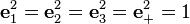 and
and  , where the space is denoted
  and its algebra is denoted . The algebra is very useful and is called the conformal geometric algebra of Euclidean physical space (C3GA). Its generalization to higher dimensions is called the homogeneous model of
  [3](27). The discussion of C3GA is beyond the scope of this article, except to mention that quaternion rotation concepts are central to using C3GA, wherein operators of the form
  generate all the ordinary transformations on
  , including translations.
Clifford geometric algebra is also commonly called just geometric algebra. Geometric algebra, in the form discussed here, is introduced in the 1984 book Clifford Algebra to Geometric Calculus, A Unified Language for Mathematics and Physics[4] by authors David Hestenes and Garret Sobczyk. Geometric algebra derives from earlier work on the abstract algebras of Clifford numbers that assign little or no geometrical meanings or interpretations. The emphasis of geometric algebra is on geometrical interpretations and applications. Clifford geometric algebra is named after William Kingdon Clifford. Clifford wrote papers, including Applications of Grassmann’s Extensive Algebra (1878)[5] and On The Classification of Geometric Algebras (1876)[6], that introduced geometric algebra as a unification of the earlier geometric algebras of Argand, Möbius, Gauss, Peacock, Hamilton, Grassmann, Saint-Venant, Kirkman, Cauchy, and Peirce. Clifford died in 1879 before he could fully develop and publish his ideas on geometric algebra.
Rules for the quaternion and Euclidean vector units
While the quaternion units have the rule or formula , the Clifford units of have the formula
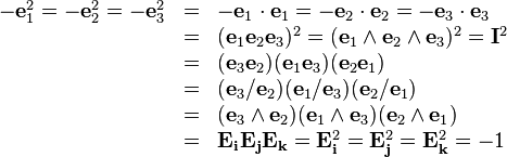
which is also showing some extra identities that map to quaternion quadrantal versors. The quaternion units map into as the Euclidean vector biradials, which are called unit bivectors or -blades in Clifford algebra
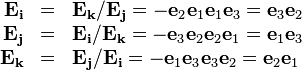
and it is seen that, in terms of the quotients, the mapping is quite simple when we view the quaternion units as quadrantal versor rotation axes being held in right-hand on right-handed axes model, or held in left-hand on left-handed axes model while fingers curl round the rotational direction as thumb points in the positive direction of the axis. The inverse of a quaternion unit is its negative or conjugate, while the inverse of a Euclidean unit is itself. The square of a unit bivector is , as for example  .
.
For  , different units multiply anti-commutatively
 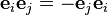 and are identical to their outer product
 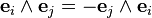 , where the outer product symbol
  between different base vector units is only synonymous or symbolic of their perpendicularity, or of a angle between the units. The inner product symbol
  between same base vector units is again only synonymous or symbolic of their parallelism, or of a zero angle between them. We also have the important fundamental geometric product of vector units
  which is a true formula since either
  and results in
 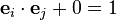 , or and results in
 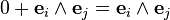 .
.
The outer product
The formulas contain the product called the outer product. The outer product of vectors has the same magnitude as the cross product  of vectors, but the result is not a vector but is a value called a -vector or bivector. It will be shown that the cross product of vectors is given by the formula
 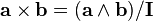 . The outer product of parallel
  vector components is zero
  , and the outer product of perpendicular
  vector components is an irreducible symbolic outer product expression of the perpendicular vector components. The outer product of vectors is a new -dimensional geometrical object representing a geometrical measure of their perpendicularity or space.
The appearance of the outer and inner product symbols between the different and same orthonormal base vector units in the rule formulas, and the relation to the value  and , can also serve to define these products in terms of simple algebraic multiplications of the units in ways consistent with the rule formula. The product of algebraic multiplication of two values in terms of only base vector units and scalars, obeying the basic rule formula, is known as the geometric product. The absence of any product symbol means algebraic multiplication consistent with rules, i.e. a geometric product.
An important result in the outer product of vectors is
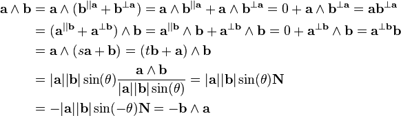
that one of the two parallel components is always arbitrarily scaled or deleted, such that or can be moved or translated parallel to or (perhaps until intersecting or becoming collinear with another object or line of interest) without affecting the result of their outer product. The value  is the irreducible unit bivector of the outer product
  . It will be shown that represents the plane containing and as a unit of directed and oriented area and that it also acts as the quadrantal versor of the plane, similar to a unit vector in quaternions.
Outer products are geometrical values for imaginaries
The outer product expression  can generally be written

where the determinant  of the matrix of vectors in an -dimensional space is the -volume of a -parallelotope formed by the -frame of the vectors . The outer product of the vector-units
  can be regarded as a type of imaginary value or symbol, representing physical perpendicularity of the unit vectors in up to
  physical dimensions, and representing imaginary perpendicularity in higher dimensions
  . Similar to the imaginary value symbol , the imaginary product symbol is irreducible to a real value by itself. However, the square of an imaginary product, such as
  , is a real value. Generally, it is shown that
![\begin{array}{rcl}
( \mathbf{e}_{1} \wedge \mathbf{e}_{2} \wedge \cdots \wedge \mathbf{e}_{n}
)^{2} & = & \left( \sqrt{-1} \right)^{2 [ n ( n-1 ) /2 ]} = ( -1 )^{n ( n-1
) /2} = \pm 1\\
( 1,2,3,4,5,6, \ldots ,n ) & \rightarrow & ( +1,+1,-1,-1,+1,+1, \ldots , \pm
1 )\end{array}](../I/m/8032f9394c28c6f9b1ce738f18f64b3a.png)
holds good for base unit vectors of an -dimensional Euclidean space where  . Taking square roots, we might (but should not) write
  and find that the right side has lost all of the vectors or axes of the left side (a geometrical value), and that the right side is generally a kind of complex number (a metrical value). However, this direct identification of a geometrical value to a metrical value is not valid. Nevertheless, it can be said that the geometrical -parallelotope unit may represent a particular extension or instance of the ordinary complex number symbol when
  , and of the split-complex or hyperbolic number symbol
  when
when  . Multivectors of the form
  , being a scalar
  plus -blade, behave either as ordinary complex values on a complex plane or as hyperbolic values on a hyperbolic plane. The unit -parallelotopes
  can be interpreted as geometrically specific objects that represent the metrical values and which by themselves represent unknown, lost, or arbitrary geometrical objects. Similar to quaternions and losing an axis of rotation at angles and , it could be a problem to lose a -blade or -vector used as a representation of a quaternion vector or axis of rotation.
Outer product is identified with scalar multiplication
The outer product with scalars is identical to ordinary scalar multiplication. Scalars are considered to be perpendicular to all values, including to another scalar so that  represents the -volume of an unknown -parallelotope. It is not certain that
  is an area since an area is represented by
  , the outer product of two vectors. All we can say about is that it is a scalar product, or pure inner product (this may seem to be a backwards statement), or pure measure of parallelism between geometrical objects in the same dimensions by non-zero amounts, or the result of a geometrical object contracted to zero dimensions by inner product with another geometrical object. Contraction is the generalization of the vector dot product to dot products of higher-dimensional (or grade) geometrical objects represented by outer product expressions. An outer product
  of scalars
  can be reduced to
  , where
  and it represents an identity matrix that has lost its vectors and has an indeterminate dimension, or has become dimensionless (non-vectorial) and allowed to be identical to the unit
  -vector .
As an additional comment, it should be noted that the formulas for the inner and outer products with scalars have not been fully agreed upon by all mathematicians in geometric algebra[7](247). New or alternative formulas are beyond the scope of this article. Most of the currently available software for geometric algebra continues to use the rules that the inner product with a scalar is zero, and the outer product with a scalar is identical to ordinary scalar multiplication, and these are the rules followed in this article.
A proposed change to the inner product says that the new inner product with a scalar is to be also identical to scalar multiplication, giving the formulas[7](279)
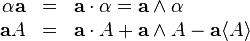
where  is any scalar, is any vector, and is any multivector. If the multivector contains a scalar component, represented by the scalar grade selector
  , then
  subtracts one of the two copies. If
  , where
  is a blade (no scalar component), then the “Chevalley formula”

continues to be valid. However, in general the Chevalley formula with any multivector is no longer valid under this change. This proposed change is essentially the same as the (fat) dot product, but it tries not to introduce a new product symbol.
Grades, blades, and vectors
The outer product expressions  ,
,  , , and
  represent, respectively, the geometrical values or objects: a -blade or metrical scalar
  in a -dimensional scalar subspace, a -vector or geometrical vector directed-length
  in the -line, a -vector or geometrical bivector directed-area of parallelogram in the -plane (or -plane), and a -vector or geometrical trivector directed-volume of parallelepiped in the
  -space (or -space).
A sum of linearly independent  -blades is called a -vector, where the number is called the grade. The three vector units are the unit -blades and their linear combinations are grade- vectors in a -dimensional subspace of . The three unit -blades are
  ,
,  , and
, and  , and a -vector has the general form
  representing a pure quaternion vector or grade- vector in a -dimensional subspace of . The single unit -blade
  , called the unit pseudoscalar, is a grade- vector in a -dimensional subspace of . There is a total of
  -blade dimensions in .
The outer product of a  -blade and -blade is a
  -blade, or if any vector is common between the blades multiplied since they do not span any area or volume (no perpendicular component).
A multivector is a sum or linear combination of linearly independent -vectors of various grades .
There are no -blades or larger outer product expressions or objects than the 3-blade pseudoscalar in , since there are only three base vector units .
Outer product expressions construct representations of directed geometric objects or values that are within a certain attitude (a space spanned by a set of unit -vectors), have a positive scalar magnitude, and have a direction or orientation (relative to the attitude or space) that is represented by a positive or negative sign on the magnitude.
The value of an outer product expression can also be represented by a matrix containing the vectors as elements where the determinant gives the signed magnitude relative to the orientation of the basis.
The inner product
The product called the inner product is the complementary product to the outer product and is similar to the dot product of vector analysis and linear algebra, except that the inner product of quaternion vectors, if represented by 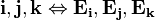 as pseudovectors, is the negative of the value given by the dot product in actual quaternions. The Clifford algebra extends the inner product to take inner products of multivectors. The inner product of parallel components is a scalar
  similar to multiplying numbers on a real or complex number line or axis, and the inner product of perpendicular components is zero
  . The inner product is a geometrical measure (a multivector) of parallelism. Between two -vectors of the same grade, the inner product reduces to a pure metrical measure (a scalar) of their parallelism, and no contracted (grade reduced) geometrical outer product expressions, objects, or vector components will remain.
An important result in the inner product of vectors is
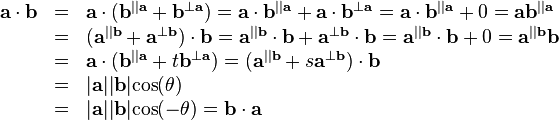
that one of the two perpendicular components is always arbitrarily scaled or deleted, such that or can be moved or translated perpendicular to or without affecting the result of their inner product.
The inner product of a -blade and -blade is a  -blade, which is often a -blade scalar. Scalars are considered to be perpendicular to all values, even to other scalars; therefore, the inner product involving a scalar factor is zero. Inner products that produce a scalar can be represented by the determinant of a matrix formed by the multiplication of two other matrices representing outer products of equal grade.
A note on terminology may be appropriate here. The “inner” and “outer” products discussed in this article are those of the Clifford geometric algebra. In the terminology of matrix linear algebra, an “inner product”, “dot product”, or “scalar product” is an ordinary matrix multiplication of a row vector with a column vector that produces a single scalar element, and is the means by which the dot product of vectors is computed in vector calculus. Also in the terminology of matrix linear algebra, the “outer product” is the multiplication of a column vector with a row vector that produces a matrix. In the terminology of Hermann Grassmann’s exterior algebra, there are “interior” and “exterior” products, which are very closely related to the Clifford geometric algebra’s inner and outer products. Geometric algebra has many distinct products to represent scalar products, inner products, outer products, dot products, contraction products, and other specialized products that can relate to products or concepts used in other algebras. Although distinct, the various products in geometric algebra are all derived from, or are parts of, the geometric product.
The geometric product of two Euclidean vectors is the sum of their inner and outer products. This is similar to the quaternion product of two pure quaternions (quaternion vectors), which is their cross product minus their dot product. The quaternion product is the geometric product for quaternions. In Clifford geometric algebra, the geometric product generalizes the quaternion product to more than four dimensions.
The sum of the inner and outer products
While the outer and inner products are of complementary magnitude according to the trigonometric functions, neither is a complete product of vectors since each deletes a parallel or perpendicular component in one of the factors. Outer and inner products are geometric measures of perpendicularity and parallelism, respectively. The complementary magnitudes suggest that they are the projected components of yet some other value that is vectorially equal to their sum
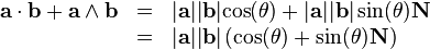
This sum appears very similar to the quaternion vector biradial 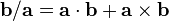 , and they can be shown to be related as duals by dividing by the unit pseudoscalar. Considering unit vectors, and quaternion vectors only on the left of
  and Euclidean vectors for the rest, we have
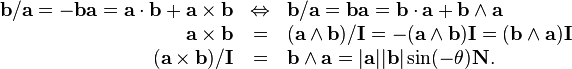
Since we started looking at the product first, the angle is now seen to represent the angle measured positive from to , and goes the reverse way from to . Unit bivector represents a quadrantal versor in the direction from to , or  and
and  . If we would agree to go back and reverse the sign on , we would have the usual rotational orientation used in quaternion rotation biradials. However, unit bivectors like do in general represent the negative rotational direction compared to the similar looking cross product. For example, in quaternions
 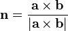 is the quadrantal rotation versor or axis that rotates from toward , while in Euclidean vectors the similar looking unit bivector
 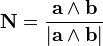 is a quadrantal versor, or geometric multiplier that effects planar rotation by , that rotates from towards , according to
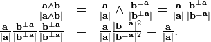
For unit vectors, the direct expression of this rotation is  . We also could again agree to reverse angles and then make
  as quadrantal versor from towards to match the Euclidean biradial where the angle would be positive from to . The choice of orientation, to measure an angle positive or negative from to or to , is the sign on the angle used in the sine function
  of the outer product and this is why
 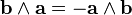 holds in general. The choice of orientation could also be viewed as a choice between axis or inverse axis, or between angle or reverse angle.
When the angle between vectors and , the product or sum  reduces to just the positive scalar
 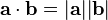 which is the expected product of parallel vectors; in quaternions, this product would be negative since quaternion vectors square negative and quaternions treat vectors as imaginary directed quantities in a space that is spanned by three imaginary units. Here, we have a real Euclidean space spanned by real units.
When , the sum reduces to  which is a directed-area parallelogram of magnitude
  in the plane of unit bivector , and so the product represents the expected geometrical object.
For other values of , the result is a multivector value where the scalar part represents the projection of the multivector onto a scalar axis, and the bivector part represents the projection of the multivector onto a bivector axis.
Since is a unit bivector, it squares to in the same way as a quaternion unit vector; and therefore, the sum of the inner and outer products of two Euclidean vectors has the form and characteristics of an ordinary complex number or a quaternion. The magnitude of this number is found by taking the square root of the product of conjugates, by which we can see that the magnitude really is . Also by similarity to complex numbers or quaternions, we know this must be the product from which the magnitudes and angle are taken. Yet, the Euclidean vectors and themselves do not have characteristics of ordinary complex numbers. Since and square positive, they do have the characteristics of split-complex numbers or hyperbolic numbers.
The multivector can be written as
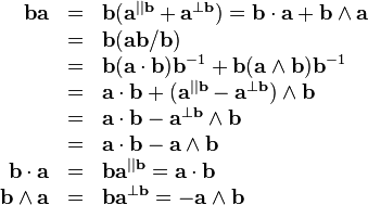
which shows more properties of the algebra, and is the reflection of the scalar and bivector components of the product in the vector . Each vector in the -blade is rotated or reflected individually, and that is the general procedure to rotate blades.
The reverse of a blade
The outer product, that constructed the bivector , has the characteristic of constructing unit blades that square  or in a certain pattern. In general, it can be shown by a sequence of anti-commutative identities, that any blade and its reverse are related by

where is the grade of the blade. The square of any -blade has the sign given by  . For
. For  , the pattern looks like
  so that at
  for , then
  .
.
The value  can represent a triangular area that is equal to the total number of bivector reverses. For example, to reverse the
  for
for  , it takes
  bivector reverses to move
  to the right side
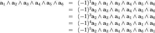
and it takes  bivector reverses, respectively, to move
  into their reversed spots. The last vector
  takes zero reverses. A triangle of these bivector reverse counts can be constructed as the triangle of numbers
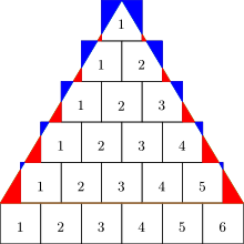
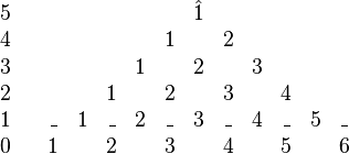
that has a total areal count of  the base
  times the height
![\begin{array}{rcl}
n ( n-1 ) /2 & = & 6 ( 6-1 ) /2\\
& = & 15\\
& = & 5+4+3+2+1\\
& = & [ n-1 ] ( [ n-1 ] +1 ) /2\end{array}](../I/m/ebb5a8a78605ab2e87e5d18fc4653e39.png)
which is the triangular number (sum of integers) formula for ![[ n-1 ] =5](../I/m/ba6ee89ea072420ad95690864fed78d0.png) .
.
The sum of integers is proved algebraically by adding the numbers counting up, plus adding the numbers counting down as follows.

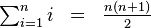
The square of a blade
In geometric algebra, squaring a blade is an important algebraic operation. It extends the concept of squaring a vector to more dimensions or to higher grades of vectors.
Consider vectors written in component form as

Using the formula for the reverse of a -blade
we can write the square of a -blade as


Using the recursive formula for the inner product of blades, we can expand this inner product as

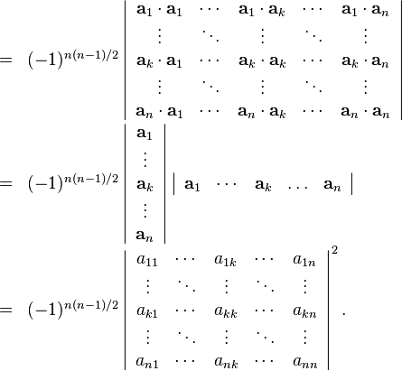
To demonstrate this result for , let’s take

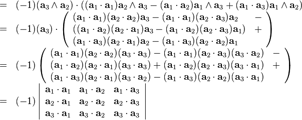
and factoring this determinant gives
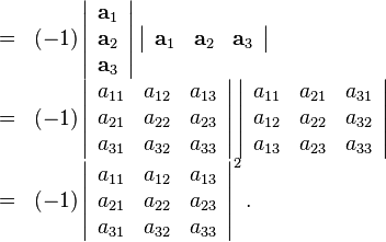
The square of a -blade has a sign given by , and has a positive magnitude, or absolute value, given by the square of the determinant of the scalar coordinates.
The determinant of the scalar coordinates
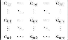
is the signed, or oriented, -volume of the directed -parallelotope framed by the vectors. Multiplying this determinant by  gives the signed -volume of the directed -simplex framed by the vectors.
It can also be seen that the product of two parallel -blades, on the same unit -blade or in the same -space, is the scalar product

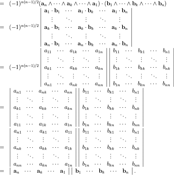
The sign factor is eliminated by reversing rows in the first determinant.
More generally, the inner product of two  -blades
  and
and  of vectors in a -dimensional base space or -space spanned by orthonormal units
  is the determinant
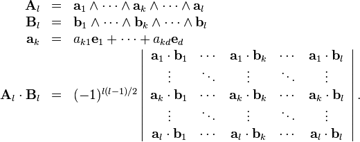
If  then this determinant can be factored into the product of two determinants, but otherwise it cannot since the factored matrices would be
  and
and  which are not square and have no determinants.
The free software SymPy, for symbolic mathematics using python, includes a Geometric Algebra Module and interactive calculator console isympy. The isympy console can be used demonstrate these results. A simple example of console interaction follows to compute the product of parallel -blades
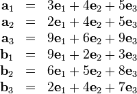

$isympy
>>> from sympy.galgebra.ga import *
>>> (e1,e2,e3) = MV.setup('e*1|2|3',metric='[1,1,1]')
>>> (a1,a2,a3) = symbols('a1 a2 a3')
>>> (b1,b2,b3) = symbols('b1 b2 b3')
>>> a1 = 3*e1 + 4*e2 + 5*e3
>>> a2 = 2*e1 + 4*e2 + 5*e3
>>> a3 = 9*e1 + 6*e2 + 9*e3
>>> b1 = 9*e1 + 2*e2 + 3*e3
>>> b2 = 6*e1 + 5*e2 + 8*e3
>>> b3 = 2*e1 + 4*e2 + 7*e3
>>> (a1^a2^a3)|(b1^b2^b3)
-102
>>> (A,B) = symbols('A B')
>>> A = Matrix([[9,6,9],[2,4,5],[3,4,5]])
>>> B = Matrix([[9,2,3],[6,5,8],[2,4,7]])
>>> A.det() * B.det()
-102
The geometric product ab of Euclidean vectors
For Euclidean vectors and , we have the products
![\begin{array}{rcl}
\mathbf{a}\mathbf{b} & = & ( a_{x} \mathbf{e}_{1} +a_{y} \mathbf{e}_{2}
+a_{z} \mathbf{e}_{3} ) ( b_{x} \mathbf{e}_{1} +b_{y} \mathbf{e}_{2} +b_{z}
\mathbf{e}_{3} )\\
& = & a_{x} b_{x} \mathbf{e}^{2}_{1} +a_{y} b_{y} \mathbf{e}^{2}_{2} +a_{z}
b_{z} \mathbf{e}^{2}_{3} +\\
& & a_{x} b_{y} \mathbf{e}_{1} \mathbf{e}_{2} +a_{x} b_{z} \mathbf{e}_{1}
\mathbf{e}_{3} +\\
& & a_{y} b_{x} \mathbf{e}_{2} \mathbf{e}_{1} +a_{y} b_{z} \mathbf{e}_{2}
\mathbf{e}_{3} +\\
& & a_{z} b_{x} \mathbf{e}_{3} \mathbf{e}_{1} +a_{z} b_{y} \mathbf{e}_{3}
\mathbf{e}_{2}\\
& = & a_{x} b_{x} +a_{y} b_{y} +a_{z} b_{z} +\\
& & ( a_{z} b_{y} -a_{y} b_{z} ) \mathbf{e}_{3} \mathbf{e}_{2} +\\
& & ( a_{x} b_{z} -a_{z} b_{x} ) \mathbf{e}_{1} \mathbf{e}_{3} +\\
& & ( a_{y} b_{x} -a_{x} b_{y} ) \mathbf{e}_{2} \mathbf{e}_{1} +\\
& = & \mathbf{a} \cdot \mathbf{b}+ \left|\begin{array}{ccc}
\mathbf{E}_{\mathbf{i}} & \mathbf{E}_{\mathbf{j}} &
\mathbf{E}_{\mathbf{k}}\\
b_{x} & b_{y} & b_{z}\\
a_{x} & a_{y} & a_{z}
\end{array}\right|\\
& = & \mathbf{a} \cdot \mathbf{b}+ ( b_{x} \mathbf{E}_{\mathbf{i}} +b_{y}
\mathbf{E}_{\mathbf{j}} +b_{z} \mathbf{E}_{\mathbf{k}} ) \times ( a_{x}
\mathbf{E}_{\mathbf{i}} +a_{y} \mathbf{E}_{\mathbf{j}} +a_{z}
\mathbf{E}_{\mathbf{k}} )\\
& = & \mathbf{a} \cdot \mathbf{b}- ( a_{x} \mathbf{E}_{\mathbf{i}} +a_{y}
\mathbf{E}_{\mathbf{j}} +a_{z} \mathbf{E}_{\mathbf{k}} ) \times ( b_{x}
\mathbf{E}_{\mathbf{i}} +b_{y} \mathbf{E}_{\mathbf{j}} +b_{z}
\mathbf{E}_{\mathbf{k}} )\\
& = & \mathbf{a} \cdot \mathbf{b}- ( \mathbf{a}/\mathbf{I} ) \times (
\mathbf{b}/\mathbf{I} ) = | \mathbf{a} | | \mathbf{b} | \left[
\mathrm{cos} ( \theta ) - \sin( \theta ) \mathbf{N} \right]\\
& = & | \mathbf{a} | | \mathbf{b} | e^{- \theta \mathbf{N}} = \mathrm{K}
( \mathbf{b}\mathbf{a} ) =\mathbf{a} \frac{\mathbf{b}^{2}}{\mathbf{b}} = |
\mathbf{b} |^{2} \mathbf{a}/\mathbf{b}\\
\mathbf{b}\mathbf{a} & = & \mathbf{b} \frac{\mathbf{a}^{2}}{\mathbf{a}} = |
\mathbf{a} |^{2} \mathbf{b}/\mathbf{a}= | \mathbf{a} | | \mathbf{b} |
e^{\theta \mathbf{N}} = \mathrm{K} ( \mathbf{a}\mathbf{b} )\end{array}](../I/m/d992caa80252116e3314dca368f781fc.png)
which are called the geometric product of vectors. The notation and concept of the quaternion conjugate  operation can be usefully adapted to the Euclidean biradials, such that where there was a pure quaternion unit vector part to take negative (as axis or angle) there is now a similar unit bivector part . The unit bivector is now being taken as quadrantal versor from toward , and angle is positive from toward .
The geometric product can also be shown to hold for any product of a vector and multivector, such as  and
and  , although the evaluation of these inner and outer products of a vector and multivector require usage of the formulas for expansion of inner and outer products. The geometric product usually has no special symbol, and the product is invoked, as shown, by spaces and juxtaposition of the values to be multiplied.
The quaternion product PQ of even-grade multivectors
The geometric product is found to be the same as the quaternion product when multiplying values that isomorphically represent quaternions in . The quaternion representation and multiplications are
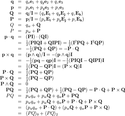
where the pseudoscalar multiplies commutatively (like a scalar) with all other values, and  , causing some changes in signs.
Dual and undual to convert to and from quaternions
Taking the dual (dividing by on the right) of the Euclidean vector  as
as  produces its pure quaternion vector representation
  . Taking the undual (multiplying by on the right) of the bivector as
  reproduces the Euclidean vector represented by the pure quaternion vector .
The inner product of quaternionic bivectors has negative sign
In the equation that represents quaternion multiplication  , the sign on
  is positive, making the equation appear different here than in the actual quaternion formula for quaternion multiplication
  that represents. Therefore,
 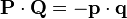 , and
, and  is the correct dot product of the undual vectors represented. This difference in sign is an issue to be aware of, but it is technically not a flaw or problem. The other values, and the values taken by grades
  and
and  , are completely consistent with quaternion multiplication.
The commutator product
The product symbol is being used in two different contexts or meanings. In  it is the Euclidean vector cross product and is the dual of the vector outer product. In
  it is called the commutator product, and is representing a quaternion vector cross product which is then taken undual to be the Euclidean vector cross product result. The commutator product is defined generally, in terms of any multivectors, by the identity

where we see this form for . For vectors, we happen to have 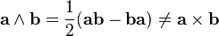 . Writing is not the commutator product; it is the vector cross product or dual of the vector outer product. The meaning of the symbol (
 ) is overloaded in the context of vectors. While outer products are associative
 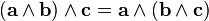 , commutator products are non-associative and obey the Jacobi identity
  . This non-associative algebra of commutator products is mostly avoided, but there is a formula
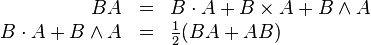
with the conditions  and
and  , that relates multiplying bivectors
  and multivectors that contain no -vector components . However, this conditional formula is of little interest for our needs.
We are only concerned with the representation of quaternions as bivectors, and the formulas of interest are the ones representing quotients and products of quaternion unit vectors, namely the biradials or versors for rotation from vector to
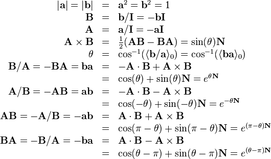
where duals  and
and  take the Euclidean vectors into quaternion representations and
  . An undual
  takes a quaternion vector
  representation back to a Euclidean vector .
Note well, that the inner product of two quaternion vectors represented as bivectors
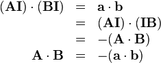
is the negative of a dot product, or inner product of two Euclidean vectors. Two quaternion vectors multiply as

and two quaternion vectors represented as bivectors multiply as

This difference in sign,  on the inner product and
  on dot product, must be paid careful attention.
Evaluating expressions in Clifford geometric algebra
The products of Clifford geometric algebra are somewhat complicated, and only careful usage of formulas and identities will give a correct evaluation. The geometric product is often written as the sum of the inner and outer products, but that formula only applies generally when at least one of the values being multiplied is a vector. Identities are used to change a product that doesn’t involve a vector into one that does, and these identities are used recursively until the product is expanded enough to complete the product evaluation using other identities for products of vectors and multivectors.
For example, the inner product  evaluates almost as if
  are merely scalars once they are arranged on the right side by using the anti-commutative multiplication identity of perpendicular vectors; the result is
  . The evaluation of the geometric product
  might at first be thought to be
  or
or  , or even
  , but it is none of them since neither operand of this geometric product is a vector. The correct evaluation using a recursive expansion identity (see identities below) is
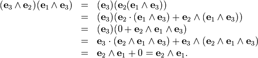
This geometric product evaluation was made more complicated by it not being a simpler product of a vector with a multivector. The evaluation of 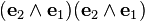 is
is
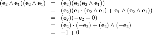
which is the correct result that matches the rule formula above. The rules or formulas applied here are listed in the identities below. Of course, these products can also be evaluated more simply by using the identities already above and applying the rule for perpendicular vectors  as needed to move values to the left or right in order to square vectors into scalars. The evaluation then looks like this
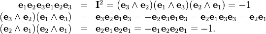
The general form of a multivector A
While looking below at some of the fundamental identities of this Clifford algebra , it may be helpful to follow along with the following additional explanations or interpretations of the values in the identities. Additional reading in the literature on Clifford geometric algebra is required to more fully understand all the concepts.
The value

is the general form of a value, called a multivector, in . The multivector has parts  called the -vector part[8](41) of , similar to taking the scalar
  and vector
  parts of a quaternion except that there are four different linearly independent parts. The number itself is called the grade, and is the grade part operator or selector on . The values in a part are also said to be of grade k or have grade k[4](3).
The part
is a real number scalar, sometimes called a 0-vector or 0-blade, and is often associated with the cosine of an angle as in quaternions.
The part

with real scalars  , is a Euclidean vector, called a 1-vector or just a vector, and its three linearly independent orthogonal components
  are called 1-blades.
The part
with real scalars  , is called a bivector (not the bivector in biquaternions) or 2-vector, and its three linearly independent orthogonal components
  are called 2-blades, and this part also represents a pure quaternion vector.
The part

with real scalar , is called a 3-vector or 3-blade, or a pseudoscalar.
There are a total of  linearly independent components or blades in all the parts of .
In a Clifford geometric algebra  with orthonormal base vector units, there are
  unique blades, and therefore the algebra has values in a -dimensional real number space. One way to see how there are unique blades is by considering the expression
where the  act as presence bits. The corresponding binary number
  has possible values. When all presence bits are zero, the resulting number is the grade-0 base unit. The grade of a blade is the sum of the presence bits. If the ordering of the units is changed in this expression, then by anti-commutativity there would only be differences in signs but no additional unique blades. The space of the blades is called the Grassmann space
  generated by the vector space
  .
.
The algebra of the even-grade parts is quaternions
The algebra of multivectors having only the even grade parts  is a closed algebra of values and isomorphic to quaternions in general, so it is a subalgebra of . The algebra of multivectors having only the odd grade parts
  is not closed since their products or quotients are in the even grade parts, which can be thought of again as quaternions as just mentioned. The product of an even part and odd part is an odd part. This relationship between odd and even parts can be notated as
  , and
, and  , and
, and  , and
, and  . If the odd parts are taken to represent only pure quaternions (vectors), letting
  , and the even parts are taken to represent only impure quaternions (quaternions with non-zero scalar part), then we will find that
  can (abstractly) represent the quaternion versor operator
 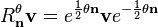 , which will take the Clifford algebra form
 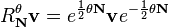 .
.
In this form, is a unit bivector that directly represents a plane of rotation, or represents a quaternion unit vector axis of rotation  , and it is the quadrantal versor of the plane represented by . The value of is still, in terms of quaternion biradials, the product or quotient of two perpendicular unit vectors. However, is now given as the product or quotient of two perpendicular Euclidean unit 1-vectors
  , or as the product or quotient of two perpendicular quaternion unit vectors represented by unit 2-vectors
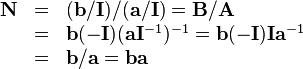
or as the dual of a unit vector rotational axis . More generally, by allowing and to again have any angle separating them, and where we had the biradial in quaternions, we now have the unit multivector of even grade
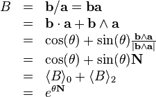
representing the same versor, and
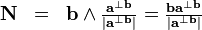
is the unit bivector of the plane of the Euclidean unit vectors to .  operates as quadrantal versor directly on Euclidean vectors in the plane of , such that
 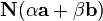 is rotated by in the plane and in the direction toward .
The reversor,

is the reverse[8](45) of denoted  .
.
The quadrantal reversor is
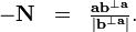
Representing a quaternion versor using an odd-grade part
It is also possible for the odd part to represent a quaternion if it takes the form
![\begin{array}{rcl}
Q\mathbf{I} & = & | Q | \left[ \mathrm{cos} ( \theta /2 ) \mathbf{I}+
\sin( \theta /2 ) \mathbf{n} \right]\\
Q & = & | Q | \left[ \mathrm{cos} ( \theta /2 ) + \sin( \theta /2 )
( \mathbf{n}/\mathbf{I} ) \right]\end{array}](../I/m/e2f47908f8f0a1f82956e59635b692d0.png)
where the Euclidean unit vector is the rotational axis, and is the rotational angle according to a right-hand or left-hand rule on right-handed or left-handed axes. A Euclidean vector can then be rotated by round as

The rotation (b/a)v(a/b) in Euclidean vectors
In general, the operation  , called taking the dual of , transforms a Euclidean planar-polar vector into an orthogonal -vector in the dual space that represents the same vector but as a quaternion axial-pole vector (also called a pseudovector) that can operate as a quadrantal versor if it has unit scale. The operation
  can be called taking the undual of . By taking the dual of Euclidean vectors to transform them into quaternions, ordinary quaternion rotation, in terms of biradials, can be performed and then the undual can be used to transform the rotated result back to a Euclidean vector. Assuming unit vectors
  , then rotation of by twice the angle from to is
![\begin{array}{rcl}
Q ( \mathbf{v}/\mathbf{I} ) Q^{-1} \mathbf{I} & = & ( [
\mathbf{b}/\mathbf{I} ] / [ \mathbf{a}/\mathbf{I} ] ) (
\mathbf{v}/\mathbf{I} ) ( [ \mathbf{b}/\mathbf{I} ] / [
\mathbf{a}/\mathbf{I} ] )^{-1} \mathbf{I}\\
& = & ( \mathbf{b} [ -\mathbf{I} ] \mathbf{a}\mathbf{I} ) ( \mathbf{v} [
-\mathbf{I} ] ) ( \mathbf{b} [ -\mathbf{I} ] \mathbf{a}\mathbf{I} )^{-1}
\mathbf{I}\\
& = & ( \mathbf{b}\mathbf{a} ) ( \mathbf{v} [ -\mathbf{I} ] ) (
\mathbf{b}\mathbf{a} )^{-1} \mathbf{I}\\
& = & ( \mathbf{b}/\mathbf{a} ) \mathbf{v} ( \mathbf{a}/\mathbf{b} )\end{array}](../I/m/2e56bd8a73035e9322f1916701ab72ee.png)
which shows that the products or quotients of Euclidean unit vectors represent quaternion versors that can directly operate on a Euclidean vector to perform a rotation in the Euclidean vector space. Therefore, it is not required to take duals to transform to quaternion representations of rotations, nor then undual any rotated results.
The following are some of the most important identities for the Clifford geometric algebra of Euclidean 3-space .
Identities: Euclidean base unit vectors
Euclidean base vector units in :
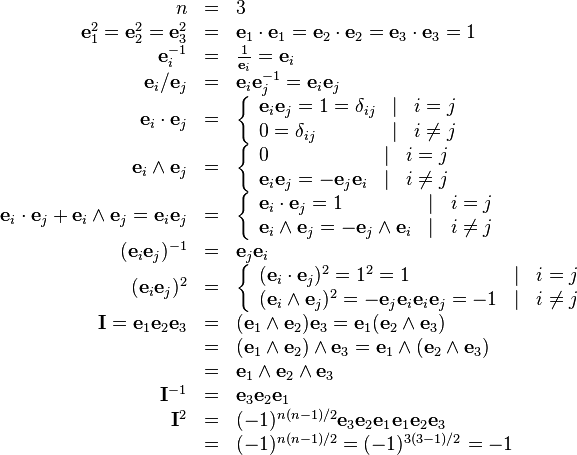
Identities: Euclidean 1-vectors
Euclidean -blades  and -vector (vector) in :
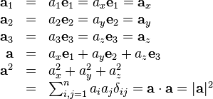
Identities: The geometric product ba of 1-vectors
The products of vectors in terms of the units. The geometric, inner, and outer products are evaluated directly in terms of the base units, and verifies that the geometric product of vectors is the sum of the inner and outer products of vectors. The outer product is found to be equal to the negative of the commutator product of their duals, which represents the negative cross product of their quaternion representations. The product is shown as a scaled versor that rotates from to :
![\begin{array}{rcl}
\mathbf{b} & = & b_{1} \mathbf{e}_{1} +b_{2} \mathbf{e}_{2} +b_{3}
\mathbf{e}_{3}\\
\mathbf{b}\mathbf{a} & = & b_{1} a_{1} +b_{1} a_{2} \mathbf{e}_{1}
\mathbf{e}_{2} +b_{1} a_{3} \mathbf{e}_{1} \mathbf{e}_{3} +\\
& & b_{2} a_{1} \mathbf{e}_{2} \mathbf{e}_{1} +b_{2} a_{2} +b_{2} a_{3}
\mathbf{e}_{2} \mathbf{e}_{3} +\\
& & b_{3} a_{1} \mathbf{e}_{3} \mathbf{e}_{1} +b_{3} a_{2} \mathbf{e}_{3}
\mathbf{e}_{2} +b_{3} a_{3}\\
& = & ( b_{1} a_{1} +b_{2} a_{2} +b_{3} a_{3} ) +\\
& & ( b_{3} a_{2} -b_{2} a_{3} ) \mathbf{e}_{3} \mathbf{e}_{2} - ( b_{3}
a_{1} -b_{1} a_{3} ) \mathbf{e}_{1} \mathbf{e}_{3} + ( b_{2} a_{1} -b_{1}
a_{2} ) \mathbf{e}_{2} \mathbf{e}_{1}\\
\mathbf{b} \cdot \mathbf{a} & = & ( b_{1} \mathbf{e}_{1} +b_{2}
\mathbf{e}_{2} +b_{3} \mathbf{e}_{3} ) \cdot ( a_{1} \mathbf{e}_{1} +a_{2}
\mathbf{e}_{2} +a_{3} \mathbf{e}_{3} )\\
& = & b_{1} a_{1} \mathbf{e}_{1} \cdot \mathbf{e}_{1} +b_{2} a_{2}
\mathbf{e}_{2} \cdot \mathbf{e}_{2} +b_{3} a_{3} \mathbf{e}_{3} \cdot
\mathbf{e}_{3}\\
& = & b_{1} a_{1} +b_{2} a_{2} +b_{3} a_{3}\\
& = & \sum_{i,j=1}^{3} b_{i} a_{j} \delta_{i j}\\
\mathbf{b} \wedge \mathbf{a} & = & ( b_{1} \mathbf{e}_{1} +b_{2}
\mathbf{e}_{2} +b_{3} \mathbf{e}_{3} ) \wedge ( a_{1} \mathbf{e}_{1} +a_{2}
\mathbf{e}_{2} +a_{3} \mathbf{e}_{3} )\\
& = & b_{1} a_{2} \mathbf{e}_{1} \wedge \mathbf{e}_{2} +b_{1} a_{3}
\mathbf{e}_{1} \wedge \mathbf{e}_{3} +\\
& & b_{2} a_{1} \mathbf{e}_{2} \wedge \mathbf{e}_{1} +b_{2} a_{3}
\mathbf{e}_{2} \wedge \mathbf{e}_{3} +\\
& & b_{3} a_{1} \mathbf{e}_{3} \wedge \mathbf{e}_{1} +b_{3} a_{2}
\mathbf{e}_{3} \wedge \mathbf{e}_{2}\\
& = & ( b_{3} a_{2} -b_{2} a_{3} ) \mathbf{e}_{3} \mathbf{e}_{2} - ( b_{3}
a_{1} -b_{1} a_{3} ) \mathbf{e}_{1} \mathbf{e}_{3} + ( b_{2} a_{1} -b_{1}
a_{2} ) \mathbf{e}_{2} \mathbf{e}_{1}\\
& = & \left|\begin{array}{ccc}
\mathbf{e}_{3} /\mathbf{e}_{2} & \mathbf{e}_{1} /\mathbf{e}_{3} &
\mathbf{e}_{2} /\mathbf{e}_{1}\\
a_{1} & a_{2} & a_{3}\\
b_{1} & b_{2} & b_{3}
\end{array}\right| = ( \mathbf{a}/\mathbf{I} ) \times (
\mathbf{b}/\mathbf{I} ) =\mathbf{A} \times \mathbf{B}\\
\mathbf{b}\mathbf{a} & = & \mathbf{b} \cdot \mathbf{a}+\mathbf{b} \wedge
\mathbf{a}=\mathbf{b} \cdot \mathbf{a}-\mathbf{B} \times \mathbf{A}\\
& = & | \mathbf{B} | | \mathbf{A} | \mathrm{cos} ( \theta ) + |
\mathbf{B} | | \mathbf{A} | \sin( \theta ) \frac{\mathbf{A}
\times \mathbf{B}}{| \mathbf{B} | | \mathbf{A} | \sin( \theta
)}\\
& = & | \mathbf{B} | | \mathbf{A} | \left[ \mathrm{cos} ( \theta ) +
\sin( \theta ) \mathbf{N} \right] = | \mathbf{B} | | \mathbf{A} |
e^{\theta \mathbf{N}}\\
& = & | \mathbf{b} | | \mathbf{a} | \left[ \mathrm{cos} ( \theta ) +
\sin( \theta ) \frac{\mathbf{b} \wedge \mathbf{a}}{| \mathbf{b} |
| \mathbf{a} | \sin( \theta )} \right]\\
& = & | \mathbf{b} | | \mathbf{a} | \left[ \mathrm{cos} ( \theta ) +
\sin( \theta ) \mathbf{N} \right]\\
& = & | \mathbf{b} | | \mathbf{a} | e^{\theta \mathbf{N}}\end{array}](../I/m/ca6bc9c1b2a41198f21fc69b1cb5e692.png)
Identities: The quaternion unit 2-vectors
Isomorphic (1 to 1) map between unit -blades and quaternion units, where the dual of a planar-polar Euclidean vector still represents but as an axial-pole quaternion vector , which is a quadrantal versor  of the plane perpendicular to if
 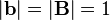 :
:
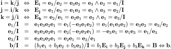
It is also important to show that the inner products of the quaternion mapping give the correct results
![\begin{array}{rcl}
\mathbf{E}_{\mathbf{i}} \cdot \mathbf{E}_{\mathbf{k}} & = & ( \mathbf{e}_{3}
\wedge \mathbf{e}_{2} ) \cdot ( \mathbf{e}_{2} \wedge \mathbf{e}_{1} )\\
& = & \mathbf{e}_{3} \cdot ( [ \mathbf{e}_{2} \cdot \mathbf{e}_{2} ]
\mathbf{e}_{1} -\mathbf{e}_{2} [ \mathbf{e}_{2} \cdot \mathbf{e}_{1} ] )
=\mathbf{e}_{3} \cdot \mathbf{e}_{1} =0\\
& = & \mathbf{E}_{\mathbf{i}} \cdot \mathbf{E}_{\mathbf{j}}
=\mathbf{E}_{\mathbf{j}} \cdot \mathbf{E}_{\mathbf{k}}\\
\mathbf{E}_{\mathbf{i}} \cdot \mathbf{E}_{\mathbf{i}} & = & ( \mathbf{e}_{3}
\wedge \mathbf{e}_{2} ) \cdot ( \mathbf{e}_{3} \cdot \mathbf{e}_{2} )\\
& = & \mathbf{e}_{3} \cdot ( [ \mathbf{e}_{2} \cdot \mathbf{e}_{3} ]
\mathbf{e}_{2} -\mathbf{e}_{3} [ \mathbf{e}_{2} \cdot \mathbf{e}_{2} ] )
=-\mathbf{e}_{3} \cdot \mathbf{e}_{3} =-1\\
& = & \mathbf{E}_{\mathbf{i}} \mathbf{E}_{\mathbf{i}}
=\mathbf{E}_{\mathbf{j}} \mathbf{E}_{\mathbf{j}} =\mathbf{E}_{\mathbf{k}}
\mathbf{E}_{\mathbf{k}}\\
\mathbf{a} \cdot \mathbf{b} & = & ( \mathbf{A}\mathbf{I} ) \cdot (
\mathbf{B}\mathbf{I} ) = \frac{1}{2} (
\mathbf{a}\mathbf{b}+\mathbf{b}\mathbf{a} )\\
& = & \frac{1}{2} (
\mathbf{A}\mathbf{I}\mathbf{B}\mathbf{I}+\mathbf{B}\mathbf{I}\mathbf{A}\mathbf{I}
) =- \frac{1}{2} ( \mathbf{A}\mathbf{B}+\mathbf{B}\mathbf{A} )\\
& = & -\mathbf{A} \cdot \mathbf{B}=-\mathbf{A} \bar{\times} \mathbf{B}\end{array}](../I/m/a9855d2675f24c759bfea50031ee2930.png)
except for a sign change, which is expected since quaternion vector units square negative or have negative signature. The vector analysis vector dot product and the geometric algebra inner product are not computed in the same way. The vector dot product is the product of a row and a column of scalar components, as in linear algebra matrix products, and ignores the vector units and their signatures. The geometric algebra inner product of blades is in the form of a Laplace expansion, as in computing determinants, and also is in terms of vector-valued factors where the signatures or squares of the vector units contribute to the result.
Cross products are
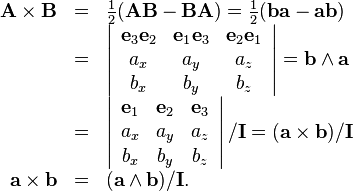
Quaternions mapped into a two dimensional space
Quaternions can be mapped into a two dimensional space with negative signatures as
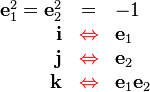
and then have the products
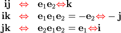
which appear to work as expected. However, there is a possible problem (hence red maps) since, while the map gives three linearly independent units, it does not give three mutually orthogonal units according to the inner products
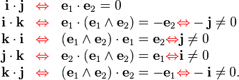
For this mapping, the inner product fails to give the desired scalar results. The vector dot product, as a matrix product of a row and a column of scalar components, can be used. The outer products are also not useful in this mapping.
The mapping of vector dot products to the negative of the anti-commutator (symmetric) products
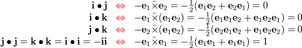
gives good results.
The mapping of vector cross products to commutator (anti-symmetric) products
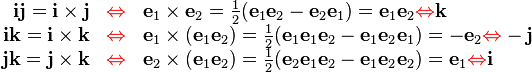
gives good results.
By combining these two good results, we can write the formula for quaternion products on this mapping as
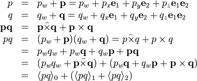
which shows that the geometric product gives all the expected quaternion results, even though the inner and outer products were not useful. For this mapping, the useful products are the geometric product and its decomposition into the anti-commutator and commutator products.
Identities: General form of multivector A by grade-k parts
General form of a multivector and its graded -vector grade- parts in :
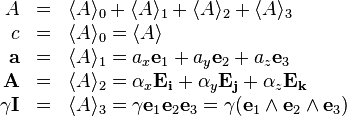
Identities: Squares, inverses, and commutative property of I
Squares, inverses, and commutative property of unit -blade pseudoscalar :
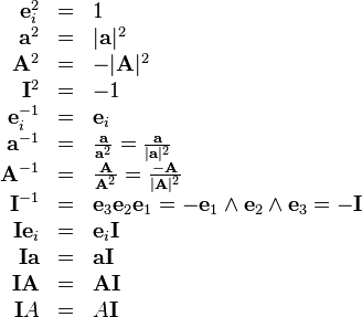
Identities: Product ba and rotation operator R
Geometric, inner, outer, and cross products of vectors and with positive angle measured from toward in the -plane (angle causes preference to give the products in order ):
Recap: The dual (dividing by the pseudoscalar or multiplying  or
or  on right side) of a Euclidean planar-polar -vector represents it as a Quaternion axial-pole -vector often useful, at the same time and with the same orientation, for rotations of both Euclidean -vectors and other vectors represented in Quaternion -vector form. The undual (multiplying on right side by ) of a -vector (representing a Quaternion vector) is a -vector that represents it as a Euclidean planar-polar vector having a positive square. The two representations of a vector by undual or dual, i.e. Euclidean -vector or Quaternion -vector, are equivalent vectors with respect to the Euclidean or Quaternion vector operations within their grades or complementary orthogonal dual spaces. The dual of a -vector and undual of a -vector can be done any time it is convenient to use the vector or bivector as Quaternion or Euclidean vector so long as appropriate care is taken not to mix incompatible formulas for one vector type with formulas for the other vector type, such as squaring since -vectors square positive and -vectors square negative. The rotation operator
  , in terms of a unit -vector , is compatible between the two such that the same operator rotates both -vectors and -vectors in the expected way within their grades. In the formulas or identities below, the dual and undual are used in the way just described, and this may allow easier understanding of how the formulas are derived and work. For example, the planar-polar Eucliden -vector
  can partially (four possible angles , , ,
  ) represent rotation
  from toward , and its dual

also partially represents that rotation as a Quaternion axial-pole -vector. The bivector can always be created as where is the Euclidean unit vector axis of rotation. Also notable is that the vector cross product is computed by a determinant of exactly the same form as in quaternions or vector analysis by using the direct mapping (not duals)  ,
,  ,
,  in the determinant.
![\begin{array}{rcl}
\mathbf{b}\mathbf{a} & = & \frac{1}{2} (
\mathbf{b}\mathbf{a}+\mathbf{a}\mathbf{b} ) + \frac{1}{2} (
\mathbf{b}\mathbf{a}-\mathbf{a}\mathbf{b} )\\
& = & \mathbf{b} \cdot \mathbf{a}+\mathbf{b} \wedge \mathbf{a}\\
& = & | \mathbf{b} | | \mathbf{a} | \mathrm{cos} ( \theta ) + |
\mathbf{b} | | \mathbf{a} | \sin ( \theta ) \mathbf{N}\\
& = & | \mathbf{b} | | \mathbf{a} | \left[ \mathrm{cos} ( \theta ) +
\sin( \theta ) \mathbf{N} \right] = | \mathbf{b} | | \mathbf{a} |
e^{\theta \mathbf{N}}\\
& = & \mathrm{K} ( \mathbf{a}\mathbf{b} )\\
\mathbf{b} \cdot \mathbf{a} & = & \frac{1}{2} (
\mathbf{b}\mathbf{a}+\mathbf{a}\mathbf{b} ) = | \mathbf{b} | | \mathbf{a}
| \mathrm{cos} ( \theta )\\
& = & | \mathbf{b} | | \mathbf{a} | \mathrm{cos} ( - \theta )
=\mathbf{a} \cdot \mathbf{b}\\
& = & \sum_{i,j=1}^{3} b_{i} a_{j} \delta_{i j} =b_{1} a_{1} +b_{2} a_{2}
+b_{3} a_{3}\\
\mathbf{b} \wedge \mathbf{a} & = & \frac{1}{2} (
\mathbf{b}\mathbf{a}-\mathbf{a}\mathbf{b} ) = | \mathbf{b} | | \mathbf{a}
| \sin( \theta ) \frac{\mathbf{b} \wedge \mathbf{a}}{| \mathbf{b}
| | \mathbf{a} | \sin( \theta )} = | \mathbf{b} | |
\mathbf{a} | \sin( \theta ) \mathbf{N}\\
& = & - | \mathbf{b} | | \mathbf{a} | \sin( - \theta )
\mathbf{N}=-\mathbf{a} \wedge \mathbf{b}\\
& = & \mathbf{b} \wedge ( \mathbf{a}^{||\mathbf{b}} +\mathbf{a}^{\bot
\mathbf{b}} ) =\mathbf{b} \wedge \mathbf{a}^{\bot \mathbf{b}}
=\mathbf{b}\mathbf{a}^{\bot \mathbf{b}}\\
& = & ( \mathbf{b}^{||\mathbf{a}} +\mathbf{b}^{\bot \mathbf{a}} ) \wedge
\mathbf{a}=\mathbf{b}^{\bot \mathbf{a}} \wedge \mathbf{a}=\mathbf{b}^{\bot
\mathbf{a}} \mathbf{a}\\
& = & ( \mathbf{a} \times \mathbf{b} ) /\mathbf{I}= ( \mathbf{a}/\mathbf{I}
) \times ( \mathbf{b}/\mathbf{I} )\\
& = & \left|\begin{array}{ccc}
\mathbf{e}_{1} /\mathbf{I} & \mathbf{e}_{2} /\mathbf{I} & \mathbf{e}_{3}
/\mathbf{I}\\
a_{1} & a_{2} & a_{3}\\
b_{1} & b_{2} & b_{3}
\end{array}\right| = \left|\begin{array}{ccc}
\mathbf{e}_{3} \mathbf{e}_{2} & \mathbf{e}_{1} \mathbf{e}_{3} &
\mathbf{e}_{2} \mathbf{e}_{1}\\
a_{1} & a_{2} & a_{3}\\
b_{1} & b_{2} & b_{3}
\end{array}\right|\\
\mathbf{a} \times \mathbf{b} & = & ( \mathbf{b} \wedge \mathbf{a} )
\mathbf{I}= ( \mathbf{a} \wedge \mathbf{b} ) /\mathbf{I}\\
& = & [ ( \mathbf{a}/\mathbf{I} ) \times ( \mathbf{b}/\mathbf{I} ) ]
\mathbf{I}= \frac{1}{2} ( \mathbf{b}\mathbf{a}-\mathbf{a}\mathbf{b} )
\mathbf{I}= \frac{1}{2} ( \mathbf{a}\mathbf{b}-\mathbf{b}\mathbf{a} )
/\mathbf{I}\\
& = & \left|\begin{array}{ccc}
\mathbf{e}_{1} /\mathbf{I} & \mathbf{e}_{2} /\mathbf{I} & \mathbf{e}_{3}
/\mathbf{I}\\
a_{1} & a_{2} & a_{3}\\
b_{1} & b_{2} & b_{3}
\end{array}\right| \mathbf{I}= \left|\begin{array}{ccc}
\mathbf{e}_{3} /\mathbf{e}_{2} & \mathbf{e}_{1} /\mathbf{e}_{3} &
\mathbf{e}_{2} /\mathbf{e}_{1}\\
a_{1} & a_{2} & a_{3}\\
b_{1} & b_{2} & b_{3}
\end{array}\right| \mathbf{I}\\
& = & \left|\begin{array}{ccc}
\mathbf{e}_{1} & \mathbf{e}_{2} & \mathbf{e}_{3}\\
a_{1} & a_{2} & a_{3}\\
b_{1} & b_{2} & b_{3}
\end{array}\right|\\
R^{\theta}_{\mathbf{N}} \mathbf{v} & = & ( \mathbf{b}\mathbf{a}
)^{\frac{1}{2}} ( \mathbf{v} ) ( \mathbf{b}\mathbf{a} )^{- \frac{1}{2}} = (
\mathbf{b}/\mathbf{a} )^{\frac{1}{2}} ( \mathbf{v} ) ( \mathbf{a}/\mathbf{b}
)^{\frac{1}{2}} =e^{\frac{1}{2} \theta \mathbf{N}} ( \mathbf{v} ) e^{-
\frac{1}{2} \theta \mathbf{N}}\end{array}](../I/m/acbece792e4a69c72b36f1123ecc281c.png)
Identities: Vector multivector products aB and Ab
Inner product with a scalar is zero, and outer product with scalar is the same as scalar multiplication.
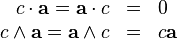
In the following,  denotes that
  is an odd integer, and
  denotes that is an even integer.
For vector and s-blade  their products are
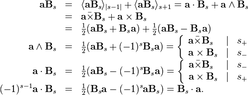
For r-blade  and vector their products are
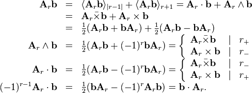
For the geometric product  of vector and multivector , the vector distributes into and multiplies with each blade within .
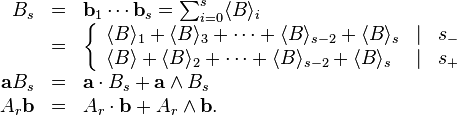
More generally, a multivector is not always a product of vectors and may contain terms or parts of any grade. See also, the recursive formula for the inner product of blades.
Operator precedence convention for ambiguous products
The otherwise ambiguous products
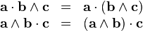
or take these meanings of products (or operator precedence) since vectors and outer products are the geometrical objects most often being operated on, measured, or compared by inner products.
The products
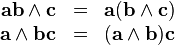
take these meanings for a similar reason.
Another operator precedence is
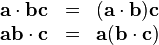
and since the inner product is a scalar factor that is seen frequently.
Identities: Projection and rejection operators for vectors
Projection, rejection, and orthogonalization operations:
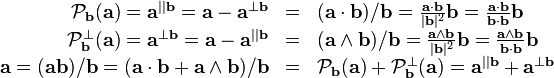
Associative, distributive algebraic properties of products
Algebraic properties of multivector products:
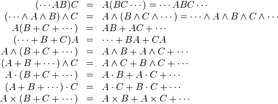
Recursive formulas for the inner products of blades
These formulas, although not entirely simple, are very important in Clifford algebra, so we will try to elaborate on them and include examples. With mastery, these formulas can find frequent practical use in algebraic operations, making it easier to derive and understand many identities.
Consider an -blade  and an -blade
  in a Clifford geometric algebra
  having base vector units
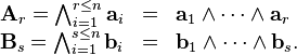
Their inner product is defined as the grade  part of their geometric product

The inner product is always a grade-reducing product. This definition of the inner product does not provide any immediately useful identities. We seek formulas for this inner product that gives useful identities.
The formula for the expansion of the geometric product of blades (EGPB) can be used to expand the inner product as
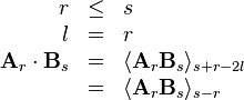
or
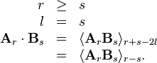
For  and
and  , EGPB gives the expansion


where  is the first partition of of grade taken in the th cyclic permutation (circular shift left) of the vectors in . The blade
  is the th second partition of grade
  . If is odd then the terms are all positive, and if is even then the terms alternate in sign.
For  , EGPB gives the similar expansion

where  is of grade
  and
and  is grade
  and are the partitions of the th cyclic permutation of the vectors in the blade . Again, the summation terms are all positive sign if is odd and have alternating signs if is even.
In each term of the summations, the inner product of two -blades can be evaluated as a determinant similar to a Gram determinant with sign factor  , as shown in the section on the square of a blade.
The EGPB formula gives an immediate expansion result with no intermediate algebraic steps or identities. To gain more identities, we can run the single expansions above in multiple steps, by repeated applications of the EGPB as follows.
It can be shown (by properties of determinants or by other means) that for 
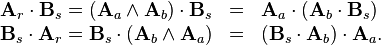
These formulas are known as the inner product reduction formulas. By these formulas, we can write the inner product of two blades in many ways by choosing any  and such that
  . Recursively, could be written as a sum, and the inner product could be further partitioned or broken into more steps and different identities. The formulas can also be used in reverse to combine nested inner product factors back into inner products of larger blades.
For  , we have the inner product of a vector and a blade and applications of the EGPB formula such as
![\begin{array}{rcl}
1 & \leq & s\\
l = r & = & 1\\
\mathbf{a} \cdot \mathbf{B}_s & = & \langle \mathbf{a}\mathbf{B}_s
\rangle_{s + r - 2 l}\\
& = & \langle \mathbf{a}\mathbf{B}_s \rangle_{s - 1}\\
& = & \sum_{k = 1}^s (- 1)^{(s - 1) (k - 1)} (\mathbf{a} \cdot
\mathbf{B}_{s (1)_k}) \mathbf{B}_{s (2)_k}\\
& = & \sum^s_{k = 1} (- 1)^{(k - 1)} (\mathbf{a} \cdot \mathbf{b}_k)
[\mathbf{B}_s \backslash\mathbf{b}_k]\end{array}](../I/m/36685a05a6b66534190c88319fbf00c4.png)
and
![\begin{array}{rcl}
r & \geq & 1\\
l = s & = & 1\\
\mathbf{A}_r \cdot \mathbf{b} & = & \langle \mathbf{A}_r \mathbf{b}
\rangle_{r + s - 2 l}\\
& = & \langle \mathbf{A}_r \mathbf{b} \rangle_{r - 1}\\
& = & \sum_{j = 1}^r (- 1)^{(r - 1) (j - 1)} \mathbf{A}_{r (1)_j}
(\mathbf{A}_{r (2)_j} \cdot \mathbf{b})\\
& = & \sum^r_{j = 1} (- 1)^{(r - j)} [\mathbf{A}_r \backslash\mathbf{a}_j]
(\mathbf{a}_j \cdot \mathbf{b}) .\end{array}](../I/m/1c1a765831252e54eb54047d0a156625.png)
The symbol  denotes the blade with its th vector
  removed, and is used in the simple formula that always has alternating signs on the summation terms, starting with positive on the side with the vector or going into the blade to the right or to the left, respectively. For example,
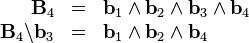
with no partitioning and no cycling.
This subsection now concludes with several examples that further explain the notation and application of the formulas.
As an example of the partitioning and cycling notation, called Sweedler’s notation, used in the EGPB formula for the general case, we have
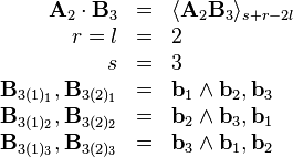
where  is the grade,
  and
and  indicate the partition number, and the small subscripted indices
  select the partitions on the three cyclic shifts left in the summation formula.
If the factors are reversed, it looks like this
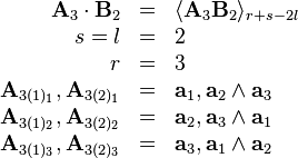
so that the partition of length  faces
faces  .
.
Example: Using the simple formula that always alternates signs, we can expand the product
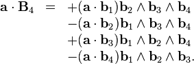
Example: Using EGPB formula that only alternates signs when the blade has even grade, we can expand the same product, noting that  is even
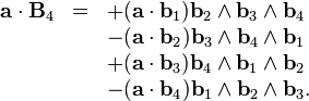
The two results are in fact equal since two bivector reverses does not alter the sign of a blade.
We can also try with an odd blade, first by simple formula
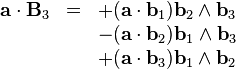
and now by the EGPB formula (with  odd, the signs are always positive)
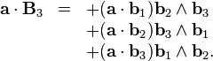
Again, the two results are equal since a bivector reverse makes a negative.
Example: Use the EGPB formula to expand
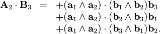
Example: By inner product reduction, use repeatedly the simplified formula for inner product of a vector and blade to expand
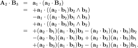
It can be checked that these are equal, but the repeated use of the simple formula reduced the terms to inner products of vectors. The check can be done using the formula
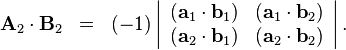
Example: Use the EGPB formula to expand
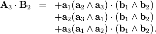
Example: Use simple formula to expand
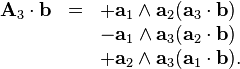
Example: Use EGPB formula to expand ( odd, all positive signs)

Expansion of the geometric product of blades
The expansion of the geometric product of blades[7](264) is more complicated than the expansion of the inner product of blades.
The following formula expands the geometric product of blades and takes a certain graded part of it.

The notation used in the summation is called Sweedler’s notation[7](30).
The selectable grade of the expansion is by steps of , by  , since the products of base units either square when equal or form a bivector when different. Any one of the possible grades in the geometric product of two blades can be selected by choosing a value for . For an -blade and -blade, the lowest possible grade in their geometric product is
  , the highest possible grade is
  , and other possible grades are between in steps of 2 grades. Setting
  makes an outer product. Setting
 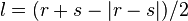 makes an inner product, and therefore this general expansion formula provides an alternative to using the recursive formula for the inner product of blades.
In a geometric algebra  with base units
  , if
, if  and/or
  then
then  and/or
  are pseudoscalars in . The geometric product of any blade with any pseudoscalar of the algebra will produce a blade in the dual space having grade . Therefore, in this case, the geometric product
 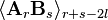 is always the inner product
  , and all the other grades that could be chosen by setting will result in zero. In summary,
 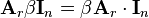 ,
, 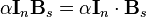 , and
, and 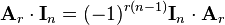 , where for the pseudoscalars commute.
Blade is partitioned  into a 2-partition of shape
  , and blade is partitioned into a 2-partition of shape
  . The first number in a partition shape is the width of a sub-blade that is referenced as a partition number , and the second number in a shape is the width of a sub-blade that is referenced as a partition number . The partition of a partitioning of is denoted
  , and the partition is denoted
  .
.
The shaped partitioning of each blade is taken on each cyclic permutation of the blade. The cyclic permutations of a blade are formed by anti-commutatively reversing bivectors within the blade until the blade is in different cyclic orders. For an -blade, there are cyclic permutations of the blade by shifting left, or rotating counter-clockwise, the vectors in the blade. As an example, the cyclic permutations of a 4-blade  are
are
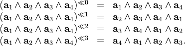
For each of these cyclic permutations we cut partitions of the specified shape. As an example, if the partition shape is  then we cut these
  partitionings
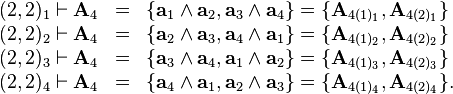
The partitionings of , per cyclic permutation, are similar and use the index  on the partitionings, while the partitionings of use the index
  .
.
As a special case, when the width of a partition is zero then that partition is set to and the blade has only that one partitioning and no permutations. This means that equals the width of the entire blade. An example is when  and , where the partitionings are

and the expansion produces a vector. An outer product with does nothing to the other factor.
The or partitionings of and the or partitionings of each have a sign of permutation
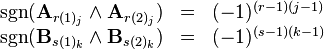
relative to the original blade due to the number of anti-commutative bivector reverses involved in each cyclic permutation. These two sign factors must be multiplied into the summation formula and evaluated for each of the  summation terms generated or expanded. They can be multiplied into partition in each partitioning so that it carries these signs of permutation into the summation. Multiplying these two factors together we can write

as the sign for the  th element of the summation. This sign formula could simply be multiplied as another factor in the summation formula to make it more explicit, but it is implied by the notation that it be carried into the summation by multiplication with a partition value.
If denotes an odd grade and is an even grade, and similarly for  and
and  , then the four different combinations of even and/or odd grades of and give the following four possible sign formulas.
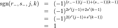
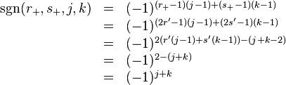
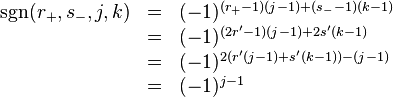
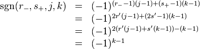
We see that, when and are both odd grades, then the sign is always positive and signs can be ignored. When the grades are both even, the signs alternate according to a Laplace expansion signs pattern, the same as the sign of a cofactor. When is even and is odd, then for every odd row the signs are all positive, and for every even row the signs are all negative. When is even and is odd, then for every odd column the signs are all positive, and for every even column the signs are all negative. Note that row and column count from and the first summation term, or row of terms, or column of terms is always positive, depending on the sign formula that matches the parities of the grades. Therefore, there is a simple pattern of the signs on summation terms depending on the parity of the grades if we follow the technique of cutting partitions on the cyclic permutations of the blades.
We can now demonstrate by some examples, to see that the formulas work as hoped.
For example, if  and , the partitionings of are
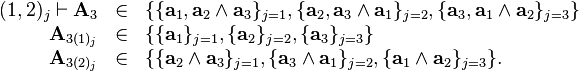
For and , the partitionings of are
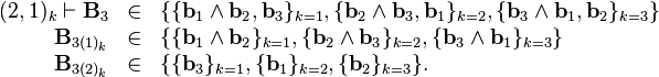
The summation holds the first partitioning of ,  and
and 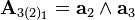 , and applies it with each of the three different partitionings of
  . This is repeated for the two other partitionings of
  , where each is also applied with each of the three partitionings of . For this example, the summation gives a sum of nine terms. Since both blades are odd, the sign formula is always .
This example expansion, with  and , produces a
  -blade or -blade

Since and  are the same grade , their grade- scalar product
  is their inner product
  .
.
This example expansion is


As another example, consider the geometric product of bivectors  . We know that bivectors in represent pseudovectors or quaternion vectors where
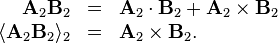
For  and
and  , the partitionings are
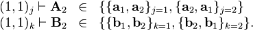
Since the two blades are even, we can use the sign formula
The expansion formula for and gives

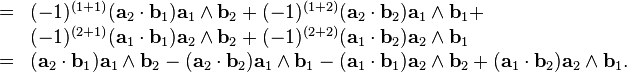
Taking and then also using the recursive formula for the expansion of inner products of blades gives

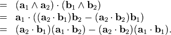
We can test these examples using the free software SymPy, for symbolic mathematics using python, which includes a Geometric Algebra Module and interactive calculator console isympy.
As a test sample for expanding the geometric product of bivectors, try the following.
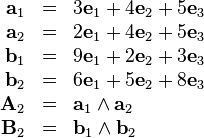
$isympy
>>> from sympy.galgebra.ga import *
>>> (e1,e2,e3) = MV.setup('e*1|2|3',metric='[1,1,1]')
>>> (a1,a2) = symbols('a1 a2')
>>> (b1,b2) = symbols('b1 b2')
>>> a1 = 3*e1 + 4*e2 + 5*e3
>>> a2 = 2*e1 + 4*e2 + 5*e3
>>> b1 = 9*e1 + 2*e2 + 3*e3
>>> b2 = 6*e1 + 5*e2 + 8*e3
>>> (A,B) = symbols('A B')
>>> A = a1^a2
>>> B = b1^b2
>>> A|B
-402
>>> (a2|b1)*(a1|b2)-(a2|b2)*(a1|b1)
-402
>>> Com(A,B)
-5*e_1^e_2 + 4*e_1^e_3 - 51*e_2^e_3
>>> Rational(1,2)*(A*B-B*A)
-5*e_1^e_2 + 4*e_1^e_3 - 51*e_2^e_3
>>> (a2|b1)*(a1^b2)-(a2|b2)*(a1^b1)-(a1|b1)*(a2^b2)+(a1|b2)*(a2^b1)
-5*e_1^e_2 + 4*e_1^e_3 - 51*e_2^e_3
To test the expansion of the geometric product of two -blades, try the following.
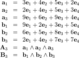
$isympy
>>> from sympy.galgebra.ga import *
>>> (e1,e2,e3,e4) = MV.setup('e*1|2|3|4',metric='[1,1,1,1]')
>>> (a1,a2,a3) = symbols('a1 a2 a3')
>>> (b1,b2,b3) = symbols('b1 b2 b3')
>>> a1 = 3*e1 + 4*e2 + 5*e3 + 2*e4
>>> a2 = 2*e1 + 4*e2 + 5*e3 + 3*e4
>>> a3 = 9*e1 + 6*e2 + 9*e3 + 4*e4
>>> b1 = 9*e1 + 2*e2 + 3*e3 + 5*e4
>>> b2 = 6*e1 + 5*e2 + 8*e3 + 6*e4
>>> b3 = 2*e1 + 4*e2 + 7*e3 + 7*e4
>>> (A,B) = symbols('A B')
>>> A = a1^a2^a3
>>> B = b1^b2^b3
>>> (A*B).grade(2)
-1196*e_1^e_2 + 874*e_1^e_3 - 162*e_1^e_4 -
 1472*e_2^e_3 + 656*e_2^e_4 - 280*e_3^e_4
>>> ((a2^a3)|(b1^b2))*(a1^b3) + \
... ((a2^a3)|(b2^b3))*(a1^b1) + \
... ((a2^a3)|(b3^b1))*(a1^b2) + \
... ((a3^a1)|(b1^b2))*(a2^b3) + \
... ((a3^a1)|(b2^b3))*(a2^b1) + \
... ((a3^a1)|(b3^b1))*(a2^b2) + \
... ((a1^a2)|(b1^b2))*(a3^b3) + \
... ((a1^a2)|(b2^b3))*(a3^b1) + \
... ((a1^a2)|(b3^b1))*(a3^b2)
-1196*e_1^e_2 + 874*e_1^e_3 - 162*e_1^e_4 -
 1472*e_2^e_3 + 656*e_2^e_4 - 280*e_3^e_4
The space was increased to four dimensions or else a product with any -blade pseudoscalar would result in a dual. In this case, the result would be a scalar. By going to four dimensions, the pseudoscalar is a -blade and the product of -blades gives a part of grade-.
For an example of mixed grades, we can expand the geometric product of a -blade  and a -blade to take the -vector part. To avoid from being a pseudoscalar, a base space of four dimensions is used again. For
  , , and , the partitionings are

Since is even and is odd, we can use the sign formula
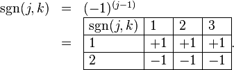
The expansion is


We can test this result as follows.
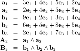
$isympy
>>> from sympy.galgebra.ga import *
>>> (e1,e2,e3,e4) = MV.setup('e*1|2|3|4',metric='[1,1,1,1]')
>>> (a1,a2) = symbols('a1 a2')
>>> (b1,b2,b3) = symbols('b1 b2 b3')
>>> a1 = 3*e1 + 4*e2 + 5*e3 + 2*e4
>>> a2 = 2*e1 + 4*e2 + 5*e3 + 3*e4
>>> b1 = 9*e1 + 2*e2 + 3*e3 + 4*e4
>>> b2 = 6*e1 + 5*e2 + 8*e3 + 5*e4
>>> b3 = 2*e1 + 4*e2 + 7*e3 + 6*e4
>>> (A,B) = symbols('A B')
>>> A = a1^a2
>>> B = b1^b2^b3
>>> (A*B).grade(3)
-62*e_1^e_2^e_3 - 125*e_1^e_2^e_4 +
 100*e_1^e_3^e_4 - 187*e_2^e_3^e_4
>>> (a2|b1)*(a1^b2^b3) + \
... (a2|b2)*(a1^b3^b1) + \
... (a2|b3)*(a1^b1^b2) - \
... (a1|b1)*(a2^b2^b3) - \
... (a1|b2)*(a2^b3^b1) - \
... (a1|b3)*(a2^b1^b2)
-62*e_1^e_2^e_3 - 125*e_1^e_2^e_4 +
 100*e_1^e_3^e_4 - 187*e_2^e_3^e_4
As a fourth example to test the fourth pattern of signs, we can expand the geometric product of a -blade and a -blade  to take the -vector part. To avoid from being a pseudoscalar, a base space of four dimensions is used again. For ,
  , and , the partitionings are

Since is odd and is even, we can use the sign formula
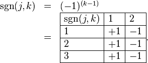
The expansion is

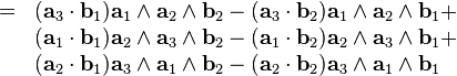
We can test this result as follows.
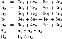
$isympy
>>> from sympy.galgebra.ga import *
>>> (e1,e2,e3,e4) = MV.setup('e*1|2|3|4',metric='[1,1,1,1]')
>>> (a1,a2,a3) = symbols('a1 a2 a3')
>>> (b1,b2) = symbols('b1 b2')
>>> a1 = 7*e1 + 6*e2 + 5*e3 + 2*e4
>>> a2 = 3*e1 + 2*e2 + 8*e3 + 3*e4
>>> a3 = 5*e1 + 7*e2 + 9*e3 + 4*e4
>>> b1 = 3*e1 + 5*e2 + 4*e3 + 5*e4
>>> b2 = 6*e1 + 4*e2 + 8*e3 + 6*e4
>>> (A,B) = symbols('A B')
>>> A = a1^a2^a3
>>> B = b1^b2
>>> (A*B).grade(3)
-348*e_1^e_2^e_3 + 1552*e_1^e_2^e_4 +
 448*e_1^e_3^e_4 + 1164*e_2^e_3^e_4
>>> (a3|b1)*(a1^a2^b2) - (a3|b2)*(a1^a2^b1) + \
... (a1|b1)*(a2^a3^b2) - (a1|b2)*(a2^a3^b1) + \
... (a2|b1)*(a3^a1^b2) - (a2|b2)*(a3^a1^b1)
-348*e_1^e_2^e_3 + 1552*e_1^e_2^e_4 +
 448*e_1^e_3^e_4 + 1164*e_2^e_3^e_4
The general expansion formula for the geometric product of two blades has been demonstrated, and the technique employed here seems to work. While being a little complicated, with practice it can get easier. There are some other expansion formulas that may be simpler or more specialized, but they often have some conditions on them that the general formula does not. The 2008 book by Hongbo Li, cited at the start of this subsection, contains details on many other expansion formulas, including a formula that further generalizes the expansion to the geometric product of more than two blades.
As a further explanation of why the expansion formula works, consider the following. See references to find formal proofs.
The expansion of an -blade  into a sum of geometric products of vectors is

If is odd then the signs are always positive, else is even and the signs alternate. For example,
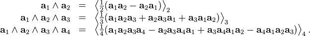
Notice that the grade can be taken on the sum, or it can be taken per term of the sum and added. Any scalar factor can be factored out of a grade selection, and constant scalars can be factored out of a summation.
Recall that, for grades and , the sign formula was written as

Using this expansion of an -blade into a sum of geometric products of vectors gives
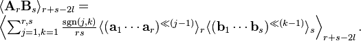
The vector products can be partitioned as

where 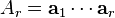 and
and 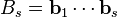 are multivectors (not blades), and are partitioned as
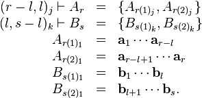
These multivectors are cyclically permutated as and increment through the summation and the partitions are taken on each permutation.
In this summation, there are nested grade selections. The inner grade selections take and grades and then multiply them geometrically. The outer grade selection takes grade  . To make the maximum inner grade, we can take this other inner grade selection

where the factor  is multiplied out by
  multiples of some average scalar product. This summation is in the form of a known corollary of the Fundamental Clifford expansion of the geometric product of vectors[7](258).
Changing geometric products to outer products in the multivectors  and
and  produces their blades and of maximum grades, and then the maximum grade in the summation is immediately given by
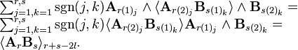
The two blades are
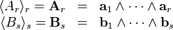
which are the grade and parts of the multivectors and .
The two blades and are still partitioned like their multivectors as
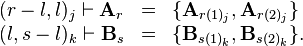
This last summation is the expansion formula for the geometric product of blades.
Another informal derivation of the expansion formula can be made as follows, and gives some additional details.
The formula for the complete anti-symmetrization of vector products produces their anti-symmetric outer products in expanded forms
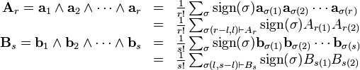
where the  (sigma) notation denotes the sum over all (not just cyclic) permutations to the order of multiplication of the vectors in the multivectors and . The value of
  is raised to the number of bivector reverses in the current permutation relative to the initial ordering of the vectors in the multivectors. The acting on the Sweedler’s notation denotes taking the partitions on each of the permutations of the vector products in the summation, which include more than just the usual (per this article) cyclic permutations. By summing over all the permutations, all of the symmetrical vector products cancel, leaving only the anti-symmetric outer product of the vectors in expanded or redundant form.
Using these complete anti-symmetrizations, we can write
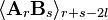
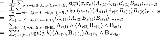
The factor  is the multiplication of the two factors from and . The first expression produces only one unique result, but there are
  copies of it which are averaged. The inner scalar product produces
  unique terms that each occur
  times and are averaged. The maximum inner grade is selected immediately by switching geometric products to outer products. In the switch, the permutations are dropped and the partitions are then taken on only the cyclic permutations, as before. The cyclic permutations produce no copies in the scalar product and the factor
  is also dropped. From there, the same expansion formula as before is obtained.
Definitions of products by graded parts of geometric product
The following are definitions of multivector products by associative, distributive, non-commutative multiplication of each component blade in with each blade in , followed by a grade selection (except for the geometric product). All products are based on selecting a certain grade of blades from the geometric product. The inner product has a special rule (to treat scalars as perpendicular to all values) that first loses or deletes any scalar part from the factors (to make sure they can’t be selected), and it produces results only of absolute grade difference ; a scalar results from inner product only when  , and if the factors are perpendicular. The scalar product simply selects the scalar part of any geometric product. The outer product also produces a scalar in the special case of the outer product of two scalars or -blades, where the grades add as
 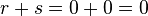 . The outer product is zero if
  where is the number of vector units of the Clifford geometric algebra (in the case considered here, with vector units ). The outer product is zero when the two blades multiplied have a common vector, since parallel vectors span zero area or volume.
Geometric product (evaluated using only rules of units; and  ):
):

Scalar product:
Inner product (standard inner product, where  for scalar ):

Outer product ( for scalar ;
  if of ):

Commutator or anti-symmetric product:
Symmetric or anti-commutator[9](55) product:

The following three products work together as a modification of the inner product.
Dot product (modified non-standard inner product, where  ):
):

Left contraction ( contraction onto ; when  the result is ):

Right contraction ( contraction by ; when  the result is ):

There are many more identities elsewhere in the literature on Clifford geometric algebras. An important concept these formulas show is that the inner product lowers grade, and outer product increases grade in definite amounts. Recognizing when a complicated expression will reduce to a scalar can sometimes save significant work, as shown some in the next subsection on the triple vector cross product.
Identities: Inner products
First, we make use of the following in the identities of this subsection:
Let  denote the reversion or reverse of an -blade , where
Properties of integer powers of :
Identity 1. Commutation of the inner product of blades. Given -blade , -blade , and the condition , then the following identity holds good:
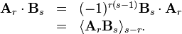
The inner product of two -blades is generally commutative: 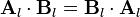 . Either is even or
  is even; therefore, the sign
  is always positive.
Proof 1. Using reversion gives
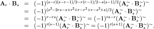
The last step, is to notice another useful identity (with no condition on it):

In this identity, the LHS and RHS inner products have the same pairing of vector inner products when recursively reduced, but they are reverses that may differ in sign. The LHS is reversed to match the sign of the RHS. This identity is also a known property of the reversion operation, usually stated generally for the entire geometric product (not just the inner product part) of any two multivectors as
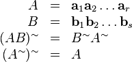
therefore  , with the inner product part included.
Identity 2. Conditional associativity of the inner product of blades. Given -blade , -blade , -blade  , and the condition
  , then the following identity holds good:
Intuitively, it is equivalent to first contract then or first then on , provided that no factors commute in the change.
The product is zero if any vector in or in is orthogonal to all vectors in . If and have any common vector then the product is again zero.
It may be tempting to drop the parentheses and just write  when the condition is satisfied. However, if Identity 1 is applied as follows, then the conditional associativity must be explicity written again such as

Therefore, writing is conditionally correct but generally incorrect and a choice of the association should be made with parentheses to avoid mistakes.
Proof 2. Using inner product commutation (Identity 1) gives
then using inner product reduction (Identity 3) in reverse gives
then using inner product commutation again gives
then using inner product reduction gives
and finally, using inner product commutation again gives
which was to be shown (Q.E.D.).
Another proof of this identity is given by Perwass[9](76) using grade projection (selection) operations.
Identity 3. Reduction of the inner product of blades. Given -blade , -blade , -blade , and condition , then the following identity holds good:

A proof of this identity is given by Perwass[9](75) using grade projections.
For , this identity, applied recursively, produces the nested inner products identity
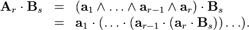
Triple vector cross product
The triple vector cross product
![\begin{array}{rcl}
\mathbf{a} \times ( \mathbf{b} \times \mathbf{c} ) & = & ( \mathbf{a} \wedge
[ ( \mathbf{b} \wedge \mathbf{c} ) /\mathbf{I} ] ) /\mathbf{I}\\
& = & ( [ ( \mathbf{c} \wedge \mathbf{b} ) \mathbf{I} ] \wedge \mathbf{a} )
\cdot \mathbf{I}\\
& = & [ ( \mathbf{c} \wedge \mathbf{b} ) \mathbf{I} ] \cdot ( \mathbf{a}
\cdot \mathbf{I} )\\
& = & [ ( \mathbf{c} \wedge \mathbf{b} ) \mathbf{I} ] \cdot (
\mathbf{I}\mathbf{a} )\\
& = & \langle ( \mathbf{c} \wedge \mathbf{b} ) \mathbf{I}
\mathbf{I}\mathbf{a} \rangle_{| 1-2 |}\\
& = & \langle ( \mathbf{b} \wedge \mathbf{c} ) \mathbf{a} \rangle_{| 1-2
|}\\
& = & ( \mathbf{b} \wedge \mathbf{c} ) \cdot \mathbf{a}\\
& = & ( \mathbf{a} \cdot \mathbf{c} ) \mathbf{b}- ( \mathbf{a} \cdot
\mathbf{b} ) \mathbf{c}\end{array}](../I/m/ef681539bbbf0b08951ac655271fd617.png)
is one of the more confusing products to evaluate in vector calculus. Here, it is converted into geometric algebra, where the inner product of blades is used to derive the expanded identity. It may be hard to see this, but the pseudoscalar commutes in the geometric product with any other value, and it also commutes across scalar, inner, and outer product symbols if it is next to the symbol. Perhaps this can be seen easier when the inner product is viewed as the geometric product (wherein clearly commutes) followed by the grade selection.
The triple cross product can also be seen as two rejections and two scaled rotations in the quaternion dual mapping where the final result is taken undual back to a Euclidean vector as
![\begin{array}{rcl}
\mathbf{b} \times \mathbf{c} & = & \left( | \mathbf{b} | e^{\frac{\pi}{2}
\frac{\mathbf{b}/\mathbf{I}}{| \mathbf{b} |}} \mathbf{c}^{\bot \mathbf{b}}
/\mathbf{I} \right) \mathbf{I}= ( \mathbf{b}/\mathbf{I} ) [ ( \mathbf{c}
\wedge \mathbf{b} ) \mathbf{b}^{-1} /\mathbf{I} ] \mathbf{I}\\
& = & \mathbf{b} ( \mathbf{b} \wedge \mathbf{c} ) \mathbf{b}^{-1}
\mathbf{I}\\
\mathbf{a} \times ( \mathbf{b} \times \mathbf{c} ) & = & \mathbf{a} (
\mathbf{a} \wedge [ \mathbf{b} ( \mathbf{b} \wedge \mathbf{c} )
\mathbf{b}^{-1} \mathbf{I} ] ) \mathbf{a}^{-1} \mathbf{I}\\
& = & \mathbf{a} ( \mathbf{a} \wedge [ ( ( \mathbf{b} \cdot \mathbf{b} )
\mathbf{c}-\mathbf{b} ( \mathbf{b} \cdot \mathbf{c} ) ) \mathbf{b}^{-1}
\mathbf{I} ] ) \mathbf{a}^{-1} \mathbf{I}\\
& = & \mathbf{a} ( \mathbf{a} \wedge [ ( \mathbf{c}\mathbf{b}-\mathbf{b}
\cdot \mathbf{c} ) \mathbf{I} ] ) \mathbf{a}^{-1} \mathbf{I}\\
& = & \mathbf{a} ( \mathbf{a} \wedge [ ( \mathbf{c} \wedge \mathbf{b} )
\cdot \mathbf{I} ] ) \mathbf{a}^{-1} \mathbf{I}\\
& = & \mathbf{a} ( \mathbf{a} \wedge [ \mathbf{c} \cdot ( \mathbf{b} \cdot
\mathbf{I} ) ] ) \mathbf{a}^{-1} \mathbf{I}\\
& = & \mathbf{a} ( \mathbf{a} \wedge [ \mathbf{c} \cdot (
\mathbf{b}\mathbf{I} ) ] ) \mathbf{a}^{-1} \mathbf{I}\\
& = & ( ( \mathbf{a} \cdot \mathbf{a} ) [ \mathbf{c} \cdot (
\mathbf{b}\mathbf{I} ) ] -\mathbf{a} ( \mathbf{a} \cdot [ \mathbf{c} \cdot (
\mathbf{b}\mathbf{I} ) ] ) ) \mathbf{a}^{-1} \mathbf{I}\\
& = & ( [ \mathbf{c} \cdot ( \mathbf{b}\mathbf{I} ) ] \cdot \mathbf{a}+ [
\mathbf{c} \cdot ( \mathbf{b}\mathbf{I} ) ] \wedge \mathbf{a}-\mathbf{a}
\cdot [ \mathbf{c} \cdot ( \mathbf{b}\mathbf{I} ) ] ) \mathbf{I}\\
& = & ( [ \mathbf{c} \cdot ( \mathbf{b}\mathbf{I} ) ] \wedge \mathbf{a} )
\cdot \mathbf{I}\\
& = & ( ( \mathbf{c} \wedge \mathbf{b} ) \cdot \mathbf{I} ) \cdot (
\mathbf{a} \cdot \mathbf{I} )\\
& = & ( ( \mathbf{c} \wedge \mathbf{b} ) \mathbf{I} ) \cdot (
\mathbf{I}\mathbf{a} )\\
& = & ( \mathbf{b} \wedge \mathbf{c} ) \cdot \mathbf{a}\\
& = & \mathbf{b} ( \mathbf{c} \cdot \mathbf{a} ) - ( \mathbf{b} \cdot
\mathbf{a} ) \mathbf{c}.\end{array}](../I/m/052bd4d4df5f643a9cecb2296dfa16ef.png)
Perhaps the above are overly-complicated ways to evaluate the triple cross product, but demonstrate different ways to view the expression. The simple way to evaluate the triple cross product is to use the recursive formula for the inner product of blades and the identity that the geometric product with a pseudoscalar is always just an inner product. Let’s also continue to assume a 3D space.

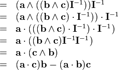
Rotation of blades
Rotating a blade is the same as rotating each vector in the blade as
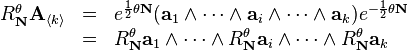
where unit bivector is the dual of a Euclidean unit vector rotation axis , or is some other unit bivector , representing a quaternion rotation axis or plane of rotation.
This result, a kind of outermorphism called versor outermorphism[9](92), is true since rotations preserve lengths and angles in rotated objects. Blade objects are rotated as rigid bodies. As an object, a blade represents a -parallelotope, or a -simplex if scaled by  .
.
In the previous section, this formula was not assumed and we had
as a rotation of a -blade. This can be evaluated and simplified as
![\begin{array}{rcl}
\mathbf{b} \times \mathbf{c} & = & \mathbf{b} ( \mathbf{b} \wedge \mathbf{c}
) \mathbf{b}^{-1} \mathbf{I}\\
& = & ( \mathbf{b}\mathbf{b}\mathbf{b}^{-1} ) \wedge (
\mathbf{b}\mathbf{c}\mathbf{b}^{-1} ) \mathbf{I}\\
& = & ( \mathbf{b} \wedge [ \mathbf{b} ( \mathbf{c}^{||\mathbf{b}}
+\mathbf{c}^{\bot \mathbf{b}} ) \mathbf{b}^{-1} ] ) \mathbf{I}\\
& = & ( \mathbf{b} \wedge [ \mathbf{c}^{||\mathbf{b}} -\mathbf{c}^{\bot
\mathbf{b}} ] ) \mathbf{I}\\
& = & ( -\mathbf{b} \wedge \mathbf{c}^{\bot \mathbf{b}} ) \mathbf{I}\\
& = & ( -\mathbf{b} \wedge \mathbf{c} ) \mathbf{I}\\
& = & ( \mathbf{b} \wedge \mathbf{c} ) /\mathbf{I}\end{array}](../I/m/37f80a20d59971f612f953c8c1d74e13.png)
giving the known formula for the vector cross product as the dual of the outer product.
References
- ↑ 1.0 1.1 1.2 1.3 1.4 1.5 Hamilton, Sir William Rowan (1853). Lectures on Quaternions: Containing a Systematic Statement of a New Mathematical Method; of which the Principles Were Communicated in 1843 to the Royal Irish Academy; and which Has Since Formed the Subject of Successive Courses of Lectures, Delivered in 1848 and Subsequent Years, in the Halls of Trinity College, Dublin: with Numerous Illustrative Diagrams, and with Some Geometrical and Physical Applications. Dublin: Hodges and Smith, Grafton-Street, Booksellers to the University. London: Whittaker & Co., Ave-Maria Lane. Cambridge: Macmillan & Co.
- ↑ J. W. Gibbs, E. B. Wilson (1929). Vector Analysis, a text-book for the use of students of mathematics and physics, founded upon the lectures of J. W. Gibbs (Sixth ed.). New Haven: Yale University Press. pp. XXII + 436.
- ↑ Gerald Sommer, ed. (2001). Geometric Computing with Clifford Algebras, Theoretical Foundations and Applications in Computer Vision and Robotics. Berlin: Springer. pp. xviii + 551.
- ↑ 4.0 4.1 David Hestenes, Garret Sobczyk (1984). Clifford Algebra to Geometric Calculus, A Unified Language for Mathematics and Physics. Fundamental Theories of Physics 5. Dordrecht-Boston-Lancaster: D. Reidel Publishing Company, a Member of the Kluwer Academic Publishers Group.
- ↑ W.K. Clifford (1882). Applications of Grassmann’s Extensive Algebra. Mathematical Papers by William Kingdon Clifford (London: Macmillan and Co.). pp. 266–276.
- ↑ W.K. Clifford (1882). On The Classification of Geometric Algebras. Mathematical Papers by William Kingdon Clifford (London: Macmillan and Co.). pp. 397–401.
- ↑ 7.0 7.1 7.2 7.3 7.4 Hongbo Li (2008). Invariant Algebras and Geometric Reasoning. Hackensack, NJ: World Scientific. pp. xiv + 518.
- ↑ 8.0 8.1 David Hestenes (1999). New Foundations for Classical Mechanics. Fundamental Theories of Physics 99 (Second ed.). Dordrecht: Kluwer Academic Publishers. pp. xi + 703.
- ↑ 9.0 9.1 9.2 9.3 Christian Perwass (2009). Geometric Algebra with Applications in Engineering. Geometry and Computing 4. Springer.