Quantum tomography

Quantum tomography or quantum state tomography is the process of reconstructing the quantum state (density matrix) for a source of quantum systems by measurements on the systems coming from the source.^[1] The source may be any device or system which prepares quantum states either consistently into quantum pure states or otherwise into general mixed states. To be able to uniquely identify the state, the measurements must be tomographically complete. That is, the measured operators must form an operator basis on the Hilbert space of the system, providing all the information about the state. Such a set of observations is sometimes called a quorum.

In quantum process tomography on the other hand, known quantum states are used to probe a quantum process to find out how the process can be described. Similarly, quantum measurement tomography works to find out what measurement is being performed.

The general principle behind quantum state tomography is that by repeatedly performing many different measurements on quantum systems described by identical density matrices, frequency counts can be used to infer probabilities, and these probabilities are combined with Born's rule to determine a density matrix which fits the best with the observations.

This can be easily understood by making a classical analogy. Let us consider a harmonic oscillator (e.g. a pendulum). The position and momentum of the oscillator at any given point can be measured and therefore the motion can be completely described by the phase space. This is shown in figure 1. By performing this measurement for a large number of identical oscillators we get a possibility distribution in the phase space (figure 2). This distribution can be normalized (the oscillator at a given time has to be somewhere) and the distribution must be non-negative. So we have retrieved a function W(x,p) which gives a description of the chance of finding the particle at a given point with a given momentum.

For quantum mechanical particles the same can be done. The only difference is that the Heisenberg’s uncertainty principle musn’t be violated, meaning that we cannot measure the particle’s momentum and position at the same time. The particle’s momentum and its position are called quadratures (see Optical phase space for more information) in quantum related states. By measuring one of the quadratures of a large number of identical quantum states will give us a probability density corresponding to that particular quadrature. This is called the marginal distribution, pr(X) or pr(P) (see figure 3). In the following text we will see that this probability density is needed to characterize the particle’s quantum state, which is the whole point of quantum tomography.

What quantum state tomography is used for

Quantum tomography is applied on a source of systems, to determine what the quantum state is of the output of that source. Unlike a measurement on a single system, which determines the system's current state after the measurement (in general, the act of making a measurement alters the quantum state), quantum tomography works to determine the state(s) prior to the measurements.

Quantum tomography can be used for characterizing optical signals, including measuring the signal gain and loss of optical devices,^[2] as well as in quantum computing and quantum information theory to reliably determine the actual states of the qubits.^[3]^[4] One can imagine a situation in which a person Bob prepares some quantum states and then gives the states to Alice to look at. Not confident with Bob's description of the states, Alice may wish to do quantum tomography to classify the states herself.

Methods of quantum state tomography

Linear inversion

Using Born's rule, one can derive the simplest form of quantum tomography. If it is known in advance that the state is represented by a pure state, a single measurement can be performed repeatedly to build up a histogram which can then be used to express the pure state in the basis of the measurement. Generally, being in a pure state is not known, and a state may be mixed. In this case, many different measurements will have to be performed, many times each. To fully reconstruct the density matrix for a mixed state in a finite-dimensional Hilbert space, the following technique may be used.

Born's rule states $\mathrm{P}(E_i | \rho) = \mathrm{Trace}(E_i \rho)$ , where $E_i$ is a particular measurement outcome projector and $\rho$ is the density matrix of the system. Given a histogram of observations for each measurement, one has an approximation $p_i$ to $\mathrm{P}(E_i | \rho)$ for each $E_i$ .

Given linear operators $S$ and $T$ , define the inner product

S \cdot T = \mathrm{Tr}[S^\dagger T] = \vec{S}^\dagger \vec{T}

where $\vec{T}$ is representation of the $T$ operator as a column vector and $\vec{S}^\dagger$ a row vector such that $\vec{S}^\dagger \vec{T}$ is the inner product in $\mathbb{C}^d$ of the two.

Define the matrix $A$ as

A = \begin{pmatrix} \vec E_1^\dagger \\ \vec E_2^\dagger \\ \vec E_3^\dagger \\ \vdots \end{pmatrix}

Here E_i is some fixed list of individual measurements (with binary outcomes), and A does all the measurements at once.

Then applying this to $\vec{\rho}$ yields the probabilities:

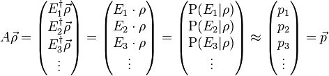A\vec{\rho} = \begin{pmatrix} E_1^\dagger \vec\rho \\ E_2^\dagger \vec\rho \\ E_3^\dagger \vec\rho \\ \vdots \end{pmatrix} = \begin{pmatrix} E_1 \cdot \rho \\ E_2 \cdot \rho \\ E_3 \cdot \rho \\ \vdots \end{pmatrix} = \begin{pmatrix} \mathrm{P}(E_1 | \rho) \\ \mathrm{P}(E_2 | \rho) \\ \mathrm{P}(E_3 | \rho) \\ \vdots \end{pmatrix} \approx \begin{pmatrix} p_1 \\ p_2 \\ p_3 \\ \vdots \end{pmatrix} = \vec{p}

Linear inversion corresponds to inverting this system using the observed relative frequencies $\vec p$ to derive $\vec \rho$ (which is isomorphic to $\displaystyle\rho$ ).

This system is not going to be square in general, as for each measurement being made there will generally be multiple measurement outcome projectors $E_i$ . For example, in a 2-D Hilbert space with 3 measurements $\sigma_x, \sigma_y, \sigma_z$ , each measurement has 2 outcomes, each of which has a projector E_i, for 6 projectors, whereas the real dimension of the space of density matrices is (2⋅2²)/2=4, leaving $A$ to be 6 x 4. To solve the system, multiply on the left by $A^T$ :

A^T A \vec\rho = A^T \vec{p}

Now solving for $\vec\rho$ yields the pseudoinverse:

\vec\rho = (A^T A)^{-1} A^T \vec{p}

This works in general only if the measurement list E_i is tomographically complete. Otherwise, the matrix $A^T A$ will not be invertible.

Continuous variables and quantum homodyne tomography

In infinite dimensional Hilbert spaces, e.g. in measurements of continuous variables such as position, the methodology is somewhat more complex. One notable example is in the tomography of light, known as optical homodyne tomography. Using balanced homodyne measurements, one can derive the Wigner function and a density matrix for the state of the light.

One approach involves measurements along different rotated directions in phase space. For each direction $\theta$ , one can find a probability distribution $w(q,\theta)$ for the probability density of measurements in the $\theta$ direction of phase space yielding the value $q$ . Using an inverse Radon transformation (the filtered back projection) on $w(q,\theta)$ leads to the Wigner function, $\mathrm{W}(x,p)$ ,^[5] which can be converted by an inverse fourier transform into the density matrix for the state in any basis.^[4] A similar technique is often used in medical tomography.

Example homodyne tomography.

Field amplitudes or quadratures with high efficiencies can be measured with photodetectors together with temporal mode selectivity. Balanced homodyne tomography is a reliable technique of reconstructing quantum states in the optical domain. This technique combines the advantages of the high efficiencies of photodiodes in measuring the intensity or photon number of light, together with measuring the quantum features of light by a clever set-up called the homodyne tomography detector. This is explained by the following example. A laser is directed onto a 50-50% beamsplitter, splitting the laserbeam into two beams. One is used as local oscillator (LO) and the other is used to generate photons with a particular quantum state. The generation of quantum states can be realized, e.g. by directing the laser beam through a frequency doubling crystal ^[6] and then onto a parametric down-conversion crystal. This crystal generates two photons in a certain quantum state. One of the photons is used as a trigger signal used to trigger (start) the readout event of the homodyne tomography detector. The other photon is directed into the homodyne tomography detector, in order to reconstruct its quantum state. Since the trigger and signal photons are entangled (this is explained by the Spontaneous parametric down-conversion article), it is important to realize, that the optical mode of the signal state is created nonlocal only when the trigger photon impinges the photodector (of the trigger event readout module) and is actually measured. More simply said, it is only when the trigger photon is measured, that the signal photon can be measured by the homodyne detector.

Now let us consider the homodyne tomography detector as depicted in figure 4. The signal photon (this is the quantum state we want to reconstruct) interferes with the local oscillator, when they are directed onto a 50-50% beamsplitter. Since the two beams originate from the same so called master laser, they have the same fixed phase relation. The local oscillator must be intense, compared to the signal so it provides a precise phase reference. The local oscillator is so intense, that we can treat it classically (a = α) and neglect the quantum fluctuations. The signal field is spatially and temporally controlled by the local oscillator, which has a controlled shape. Where the local oscillator is zero, the signal is rejected. Therefore, we have temporal-spatial mode selectivity of the signal. The beamsplitter redirects the two beams to two photodetectors. The photodetectors generate an electric current proportional to the photon number. The two detector currents are subtracted and the resulting current is proportional to the electric field operator in the signal mode, depended on relative optical phase of signal and local oscillator.

Since the electric field amplitude of the local oscillator is much higher than that of the signal the intensity or fluctuations in the signal field can be seen. The homodyne tomography system functions as an amplifier. The system can be seen as an interferometer with such a high intensity reference beam (the local oscillator) that unbalancing the interference by a single photon in the signal is measurable. This amplification is well above the photodetectors noise floor.

The measurement is reproduced a large number of times. Then the phase difference between the signal and local oscillator is changed in order to ‘scan’ a different angle in the phase space. This can be seen from figure 4. The measurement is repeated again a large number of times and a marginal distribution is retrieved from the current difference. The marginal distribution can be transformed into the density matrix and/or the Wigner function. Since the density matrix and the Wigner function give information about the quantum state of the photon, we have reconstructed the quantum state of the photon.

The advantage of this method is that this arrangement is insensitive to fluctuations in the frequency of the laser.

The quantum computations for retrieving the quadrature component from the current difference are performed as follows.

The photon number operator for the beams striking the photodetectors after the beamsplitter is given by:

\hat n_{i}=\hat a_{i}^\dagger \hat a_{i}

where i is 1 and 2, for respectively beam one and two. The mode operators of the field emerging the beamsplitters are given by:

\hat a_{1}= 2^{-1/2}(\hat\alpha - \alpha_{LO})

\hat a_{2}= 2^{-1/2}

(\hat\alpha + \alpha_{LO})

The $\hat a$ denotes the annihilation operator of the signal and alpha the complex amplitude of the local oscillator. The number of photon difference is eventually proportional to the quadrature and given by:

\hat n_{21}=\hat n_{2} - \hat n_{1} = \alpha^*_{LO} \hat a + \alpha_{LO} \hat a^\dagger

Rewriting this with the relation:

\hat q=2^{-1/2}(\hat a^\dagger+\hat a)

Results in the following relation:

\hat n_{21}=2^{1/2}|\hat\alpha_{LO}|\hat q_{\theta}

where we see clear relation between the photon number difference and the quadrature component $\hat q_{\theta}$ . By keeping track of the sum current, one can recover information about the local oscillator’s intensity, since this is usually an unknown quantity, but an important quantity for calculating the quadrature component $\hat q_{\theta}$ .

Problems with linear inversion

One of the primary problems with using linear inversion to solve for the density matrix is that in general the computed solution will not be a valid density matrix. For example, it could give negative probabilities or probabilities greater than 1 to certain measurement outcomes. This is particularly an issue when fewer measurements are made.

Another issue is that in infinite dimensional Hilbert spaces, an infinite number of measurement outcomes would be required. Making assumptions about the structure and using a finite measurement basis leads to artifacts in the phase space density.^[4]

Maximum likelihood estimation

Maximum likelihood estimation (also known as MLE or MaxLik) is a popular technique for dealing with the problems of linear inversion. By restricting the domain of density matrices to the proper space, and searching for the density matrix which maximizes the likelihood of giving the experimental results, it guarantees the state to be theoretically valid while giving a close fit to the data. The likelihood of a state is the probability that would be assigned to the observed results had the system been in that state.

Suppose the measurements $\{|y_j\rang \lang y_j|\}$ have been observed with frequencies $f_j$ . Then the likelihood associated with a state $\hat\rho$ is

L(\hat\rho) = \prod_j \lang y_j|\hat\rho|y_j\rang^{f_j}

where $\lang y_j|\hat\rho|y_j\rang$ is the probability of outcome $y_j$ for the state $\hat\rho$ .

Finding the maximum of this function is non-trivial and generally involves iterative methods.^[7]^[8] The methods are an active topic of research.

Problems with maximum likelihood estimation

Maximum likelihood estimation suffers from some less obvious problems than linear inversion. One problem is that it makes predictions about probabilities that cannot be justified by the data. This is seen most easily by looking at the problem of zero eigenvalues. The computed solution using MLE often contains eigenvalues which are 0, i.e. it is rank deficient. In these cases, the solution then lies on the boundary of the n-dimensional Bloch sphere. This can be seen as related to linear inversion giving states which lie outside the valid space (the Bloch sphere). MLE in these cases picks a nearby point that is valid, and the nearest points are generally on the boundary.^[3]

This is not physically a problem, the real state might have zero eigenvalues. However, since no value may be less than 0, an estimate of an eigenvalue being 0 implies that the estimator is certain the value is 0, otherwise they would have estimated some $\epsilon$ greater than 0 with a small degree of uncertainty as the best estimate. This is where the problem arises, in that it is not logical to conclude with absolute certainty after a finite number of measurements that any eigenvalue (that is, the probability of a particular outcome) is 0. For example, if a coin is flipped 5 times and each time heads was observed, it does not mean there is 0 probability of getting tails, despite that being the most likely description of the coin.^[3]

Bayesian methods

Bayesian mean estimation (BME) is a relatively new approach which addresses the problems of maximum likelihood estimation. It focuses on finding optimal solutions which are also honest in that they include error bars in the estimate. The general idea is to start with a likelihood function and a function describing the experimenter's prior knowledge (which might be a constant function), then integrate over all density matrices using the product of the likelihood function and prior knowledge function as a weight.

Given a reasonable prior knowledge function, BME will yield a state strictly within the n-dimensional bloch sphere. In the case of a coin flipped N times to get N heads described above, with a constant prior knowledge function, BME would assign $\scriptstyle\frac{1}{N+2}$ as the probability for tails.^[3]

BME provides a high degree of accuracy in that it minimizes the operational divergences of the estimate from the actual state.^[3]

Methods for incomplete data

The number of measurements needed for a full quantum state tomography for a multi-particle system scales exponentially with the number of particles, which makes such a procedure impossible even for modest system sizes. Hence, several methods have been developed to realize quantum tomography with fewer measurements.

The concept of matrix completion and compressed sensing have been applied to reconstruct density matrices from an incomplete set of measurements (that is, a set of measurements which is not a quorum). In general, this is impossible, but under assumptions (for example, if the density matrix is a pure state, or a combination of just a few pure states) then the density matrix has fewer degrees of freedom, and it may be possible to reconstruct the state from the incomplete measurements.^[9]

Permutationally Invariant Quantum Tomography^[10] is a procedure that has been developed mostly for states that are close to being permutationally symmetric, which is typical in nowadays experiments. For two-state particles, the number of measurements needed scales only quadratically with the number of particles. ^[11] Besides the modest measurement effort, the processing of the measured data can also be done efficiently: It is possible to carry out the fitting of a physical density matrix on the measured data even for large systems. ^[12] Permutationally Invariant Quantum Tomography has been combined with compressed sensing in a six-qubit photonic experiment.^[13]

Quantum measurement tomography

One can imagine a situation in which an apparatus performs some measurement on quantum systems, and determining what particular measurement is desired. The strategy is to send in systems of various known states, and use these states to estimate the outcomes of the unknown measurement. Also known as "quantum estimation", tomography techniques are increasingly important including those for quantum measurement tomography^[14] and the very similar quantum state tomography. Since a measurement can always be characterized by a set of POVM's, the goal is to reconstruct the characterizing POVM's $\Pi_l$ . The simplest approach is linear inversion. Similar to in quantum state observation, use

\displaystyle\mathrm{Tr}[\Pi_l \rho_m] = \mathrm{P}(l | \rho_m)

Exploiting linearity as above, this can be inverted to solve for the $\Pi_l$ .

Not surprisingly, this suffers from the same pitfalls as in quantum state tomography. Namely, non-physical results, in particular negative probabilities. Here the $\Pi_l$ will not be valid POVM's, as they will not be positive. Bayesian methods as well as Maximum likelihood estimation of the density matrix can be used ^[14] to restrict the operators to valid physical results.

Quantum tomography of pre-measurement states

The main tool of the retrodictive approach of quantum physics is the pre-measurement state which allows predictions about state preparations of the measured system leading to a given measurement result. As it was shown in a recent work,^[15] such a state reveals interesting quantum properties of the corresponding measurement such as its non-classicality or its projectivity. However, we cannot realize the tomography of this state with the usual methods based on measurements, since it needs non-destructive measurements which are some particularly measurements. The experimental procedure, proposed in,^[15] is based on the retrodictive approach of quantum physics, in which we have an expression of retrodictive probabilities similar to Born's rule:

\mathrm{Pr}\left(m \vert n\right) = \mathrm{Tr}\lbrace\hat{\rho}_{retr}^{[n]}\hat{\Theta}_{m}\rbrace,

where $\hat{\rho}_{retr}^{[n]}$ and $\hat{\Theta}_{m}$ are respectively the pre-measurement state, corresponding to the measurement characterized by some a POVM element $\hat{\Pi}_{n}$ , and a hermitian and positive operator corresponding to the preparation of the measured system in a state $\hat{\rho}_{m}$ . In the frame of the mathematical foundations of quantum physics, such an operator is a proposition about the state of the system, as a POVM element, and for having an exhaustive set of propositions, these operators must be a resolution of the Hilbert space:

\sum_{m}\,\hat{\Theta}_{m}=\hat{1}.

From Born's, we can derive with Bayes' theorem,^[15]^[16] the expressions of the pre-measurement state $\hat{\rho}_{retr}^{[n]}$ and proposition operators $\hat{\Theta}_{m}$ . The pre-measurement state simply corresponds to the normalized POVM element:

\hat{\rho}_{retr}^{[n]}=\frac{\hat{\Pi}_{n}}{\mathrm{Tr}\lbrace\Pi_{n}\rbrace},

and the proposition operators are linked to the possible preparations of the system by:

\hat{\Theta}_{m}=D\mathcal{P}_{m}\hat{\rho}_{m},

where $D$ is the dimension of the Hilbert space and $\mathcal{P}_{m}$ is the probability of preparing the state $\hat{\rho}_{m}$ .

Thus, we can probe the measurement apparatus with a statistical mixture:

\hat{\rho}^{[?]}=\sum_{m}\,\mathcal{P}_{m}\hat{\rho}_{m}=\hat{1}/D,

in order to measure the retrodictive probability $\mathrm{Pr}\left(m \vert n\right)$ . This mixture could be obtained by preparations based on random choices 'm' with the probabilities $\mathcal{P}_{m}$ . Then, we replace the POVM elements describing the measurements in a usual method for the tomography of states by the operators $\hat{\Theta}_{m}$ . The method will give the state giving the probabilities $\mathrm{Pr}\left(m \vert n\right)$ which are the most closest to those measured. This is the pre-measurement state with which we can have some interesting properties of the measurement giving the result 'n', as explained in.^[15]

Quantum process tomography

Quantum process tomography (QPT) deals with identifying an unknown quantum dynamical process. The first approach, introduced in 1996 and sometimes known as standard quantum process tomography (SQPT) involves preparing an ensemble of quantum states and sending them through the process, then using quantum state tomography to identify the resultant states.^[17] Other techniques include ancilla-assisted process tomography (AAPT) and entanglement-assisted process tomography (EAPT) which require an extra copy of the system.^[18]

Each of the techniques listed above are known as indirect methods for characterization of quantum dynamics, since they require the use of quantum state tomography to reconstruct the process. In contrast, there are direct methods such as direct characterization of quantum dynamics (DCQD) which provide a full characterization of quantum systems without any state tomography.^[19]

The number of experimental configurations (state preparations and measurements) required for full quantum process tomography grows exponentially with the number of constituent particles of a system. Consequently, in general, QPT is an impossible task for large-scale quantum systems. However, under weak decoherence assumption, a quantum dynamical map can find a sparse representation. The method of compressed quantum process tomography (CQPT) uses the compressed sensing technique and applies the sparsity assumption to reconstruct a quantum dynamical map from an incomplete set of measurements or test state preparations.^[20]

Quantum dynamical maps

A quantum process, also known as a quantum dynamical map, $\mathcal{E}(\rho)$ , can be described by a completely positive map

\mathcal{E}(\rho) = \sum_i A_i \rho A_i^\dagger

where $\rho \in \mathcal{B(H)}$ , the bounded operators on Hilbert space; with operation elements $\displaystyle A_i$ satisfying $\textstyle\sum_i A_i^\dagger A_i \leq I$ so that $\mathrm{Tr}[\mathcal{E}(\rho)] \leq 1$ .

Let $\displaystyle\{E_i\}$ be an orthogonal basis for $\mathcal{B(H)}$ . Write the $\displaystyle A_i$ operators in this basis

\displaystyle A_i = \sum_{m} a_{im}E_m

This leads to

\mathcal{E}(\rho) = \sum_{m,n} \chi_{mn} E_{m} \rho E_n^\dagger

where $\chi_{mn} = \sum_{i} a_{mi} a_{ni}^*$ .

The goal is then to solve for $\displaystyle\chi$ , which is a positive superoperator and completely characterizes $\mathcal{E}$ with respect to the $\displaystyle\{E_i\}$ basis.^[18]^[19]

Standard quantum process tomography

SQPT approaches this using $d^2$ linearly independent inputs $\rho_j$ , where $d$ is the dimension of the Hilbert space $\mathcal{H}$ . For each of these input states $\rho_j$ , sending it through the process gives an output state $\mathcal{E}(\rho)$ which can be written as a linear combination of the $\rho_j$ , i.e. $\textstyle \mathcal{E}(\rho_j) = \sum_k c_{jk} \rho_k$ . By sending each $\rho_j$ through many times, quantum state tomography can be used to determine the coefficients $c_{jk}$ experimentally.

Write

E_m \rho_j E_n^\dagger = \sum_{k} B_{m,n,j,k} \rho_k

where $B$ is a matrix of coefficients. Then

\sum_k c_{jk} \rho_k = \mathcal{E}(\rho_j) = \sum_{m,n} \chi_{m,n} E_m \rho_j E_n^\dagger = \sum_{m,n}\sum_{k} \chi_{m,n} B_{m,n,j,k} \rho_k

Since $\rho_k$ form a linearly independent basis,

\displaystyle c_{jk} = \sum_{m,n}\chi_{m,n} B_{m,n,j,k}

Inverting $B$ gives $\chi$ :

\chi_{m,n} = \sum_{j,k} B^{-1}_{m,n,j,k} c_{jk}

References

↑ Quantum State Tomography. http://research.physics.uiuc.edu/QI/Photonics/Tomography/#what_is_tomography
↑ G. Mauro D’Ariano et al. Quantum tomography as a tool for the characterization of optical devices. http://www.iop.org/EJ/abstract/1464-4266/4/3/366
↑ 3.0 3.1 3.2 3.3 3.4 Robin Blume-Kohout. Optimal, reliable estimation of quantum states. http://arxiv.org/abs/quant-ph/0611080v1
↑ 4.0 4.1 4.2 A.I.Lvovsky, M.G.Raymer. Continuous-variable optical quantum state tomography. http://arxiv.org/abs/quant-ph/0511044v2
↑ K. Vogel and H. Risken. Determination of quasiprobability distributions in terms of probability distributions for the rotated quadrature phase. http://prola.aps.org/abstract/PRA/v40/i5/p2847_1
↑ Online Encyclopedia of Laser Physics and Technology. http://www.rp-photonics.com/frequency_doubling.html
↑ A I Lvovsky. Iterative maximum-likelihood reconstruction in quantum homodyne tomography. http://arxiv.org/abs/quant-ph/0311097
↑ J. Řeháček, Z. Hradil, and M. Ježek. Iterative algorithm for reconstruction of entangled states. Phys. Rev. A 63, 040303 (2001). http://prola.aps.org/abstract/PRA/v63/i4/e040303
↑ Gross, D.; Liu, Y. K.; Flammia, S.; Becker, S.; Eisert, J. (2010). "Quantum State Tomography via Compressed Sensing". Physical Review Letters 105 (15). arXiv:0909.3304. Bibcode:2010PhRvL.105o0401G. doi:10.1103/PhysRevLett.105.150401.
↑ Permutationally Invariant Quantum Tomography. http://www.pitomography.eu
↑ Tóth, G.; Wieczorek, W.; Gross, D.; Krischek, R.; Schwemmer, C.; Weinfurter, H. (2010). "Permutationally Invariant Quantum Tomography". Physical Review Letters 105 (25). arXiv:1005.3313. Bibcode:2010PhRvL.105y0403T. doi:10.1103/PhysRevLett.105.250403.
↑ Moroder, T.; Hyllus, P.; Tóth, G. Z.; Schwemmer, C.; Niggebaum, A.; Gaile, S.; Gühne, O.; Weinfurter, H. (2012). "Permutationally invariant state reconstruction". New Journal of Physics 14 (10): 105001. doi:10.1088/1367-2630/14/10/105001.
↑ Schwemmer, C.; Tóth, G.; Niggebaum, A.; Moroder, T.; Gross, D.; Gühne, O.; Weinfurter, H. (2014). "Experimental Comparison of Efficient Tomography Schemes for a Six-Qubit State". Physical Review Letters 113 (04). http://arxiv.org/abs/1401.7526. Bibcode: 2014PhRvL.113d0503S. Schwemmer, C.; Tóth, G. Z.; Niggebaum, A.; Moroder, T.; Gross, D.; Gühne, O.; Weinfurter, H. (2014). "Experimental Comparison of Efficient Tomography Schemes for a Six-Qubit State". Physical Review Letters 113 (4). doi:10.1103/PhysRevLett.113.040503.
↑ 14.0 14.1 J. Fiurasek. Maximum-likelihood estimation of quantum measurement (http://www.seedwiki.com/wiki/spie) and Review (http://arxiv.org/abs/quant-ph/0302028)
↑ 15.0 15.1 15.2 15.3 Taoufik Amri, Quantum behavior of measurement apparatus, arXiv:1001.3032 (2010).
↑ S. M. Barnett et al. arXiv:0106139 (2001).
↑ I. L. Chuang, M. A. Nielsen. Prescription for Experimental Determination of the Dynamics of a Quantum Black Box. http://arxiv.org/abs/quant-ph/9610001
↑ 18.0 18.1 J. B. Altepeter et al. Ancilla-assisted quantum process tomography. http://arxiv.org/abs/quant-ph/0303038v2
↑ 19.0 19.1 M. Mohseni, A. T. Rezakhani, D. A. Lidar. Quantum Process Tomography: Resource Analysis of Different Strategies. http://arxiv.org/abs/quant-ph/0702131
↑ Shabani, A.; Kosut, R.; Mohseni, M.; Rabitz, H.; Broome, M.; Almeida, M.; Fedrizzi, A.; White, A. (2011). "Efficient Measurement of Quantum Dynamics via Compressive Sensing". Physical Review Letters 106 (10). arXiv:0910.5498. Bibcode:2011PhRvL.106j0401S. doi:10.1103/PhysRevLett.106.100401.