Quantum superposition

Quantum mechanics
$\sigma_x \sigma_p \ge \frac{\hbar}{2}$ Uncertainty principle
Introduction Glossary History
Background Classical mechanics Old quantum theory Bra–ket notation Hamiltonian Interference
Fundamentals Complementarity Decoherence Entanglement Energy level Measurement Nonlocality Quantum number State Superposition Symmetry Tunnelling Uncertainty Wave function (collapse)
Experiments Afshar Bell's inequality Davisson–Germer Double-slit Elitzur–Vaidman Franck–Hertz Mach–Zehnder Popper Quantum eraser (delayed-choice) Schrödinger's cat Stern–Gerlach Wheeler's delayed-choice
Formulations Overview Heisenberg Interaction Matrix Phase-space Schrödinger Sum-over-histories (path integral)
Equations Dirac Klein–Gordon Pauli Rydberg Schrödinger
Interpretations Overview Bayesian Consistent histories Copenhagen de Broglie–Bohm Ensemble Hidden-variable Many-worlds Objective collapse Quantum logic Relational Stochastic Transactional
Advanced topics Quantum chaos Quantum computing Density matrix Quantum field theory Fractional quantum mechanics Quantum information science Relativistic quantum mechanics Scattering theory Quantum statistical mechanics
Scientists Aharonov Bell Blackett Bloch Bohm Bohr Born Bose de Broglie Candlin Compton Dirac Davisson Debye Ehrenfest Einstein Everett Fock Fermi Feynman Glauber Gutzwiller Heisenberg Hilbert Jordan Kramers Pauli Lamb Landau Laue Moseley Millikan Onnes Planck Rabi Raman Rydberg Schrödinger Sommerfeld von Neumann Weyl Wien Wigner Zeeman Zeilinger

Quantum superposition of states and decoherence

For any particular quantum system, the principle of quantum superposition states the existence of certain relations amongst states, respectively pure with respect to particular distinct quantum state analysers. It is a fundamental principle of quantum mechanics.

Mathematically, it refers to a property of pure state solutions to the Schrödinger equation; since the Schrödinger equation is linear, any linear combination of pure state solutions to a particular equation will also be a pure state solution of it. Such solutions are often made to be orthogonal (i.e. the vectors are at right-angles to each other), such as the energy levels of an electron. In other words, the overlap of the states is nullified, and the expectation value of an operator is the expectation value of the operator in the individual states, multiplied by the fraction of the superposition state that is "in" that state, called eigenstates. Such resolution into orthogonal components is the basis of what is known as "quantum measurement", a concept that is characteristic of quantum physics, inexplicable in classical physics.

Physically, it refers to the separation and reconstitution of different quantum states.

For example, a physically observable manifestation of superposition is interference peaks from an electron wave in a double-slit experiment.

Another example is a quantum logical qubit state, as used in quantum information processing, which is a linear superposition of the "basis states" $|0 \rangle$ and $|1 \rangle$ . Here $|0 \rangle$ is the Dirac notation for the quantum state that will always give the result 0 when converted to classical logic by a measurement. Likewise $|1 \rangle$ is the state that will always convert to 1.

Concept

The principle of quantum superposition is most clearly understood when it refers to pure states of a quantum system.

Preparation of a primary beam in a pure state

One considers a primary beam of quantal entities (examples: photons, material particles such as atoms) that has been prepared in a so-called pure state, as follows.

Initially, instances of the quantal entity of interest, ray or particle of a wave or material nature, as the case may be, are obtained in large numbers, issuing from an oven or some natural object such as the sun, that can be considered the initiating source. The source supplies a raw beam composed of a chemically pure substance (e.g. a vapour of atoms of silver) or a form of radiation (e.g. a beam of light). While they are still in the oven, the quantal entities are in some kind of mutual thermal equilibrium, having interacted with one another, directly or indirectly. Thereby they have become entangled. Also thereby, their respective quantum mechanical phases became partly coherent, for example because of stimulated emission.

A raw beam of them comes through a small hole in the wall of the oven, or a small hole in the window blind in the case of Newton using sunlight. The beam is such that, within it, interactions of the quantal entities are negligible, and the entities may be considered to some degree independent apart from their entanglement and coherence. The raw beam is passed through some sorting apparatus^[1] that will here be called a quantum filter.^[2]^[3] That is a device, such as perhaps a crystal (e.g. of calcite) or prism, that is used to select a fraction of the raw beam, very narrowly defined by some criterion used in the design of the filter. The filter is in effect a physical spectrum analyser, all the output sub-beams of which are allowed to pass to a remote place, and ignored, except one, which is the sole output sub-beam of interest, and is further processed in the experiment. (Alternatively, the filter can be such as to pass only one sub-beam, the rest of its input beam being absorbed; e.g. a piece of tourmaline.) The filter is a macroscopic object, but it is so designed and physically constructed that it can also be considered as a quantal object that has mutually entangled quantum mechanical collective modes. For example, a prism has machined smooth surfaces. Rough surfaces would not do. Likewise, the constituent microscopic particles, such as atoms, of a crystal diffractor are physically arranged with spatial periodicity.

The filtered output is here called the 'primary beam'. It is pure with respect to the filter.^[4] This means that if it is passed through a copy of the filter, it comes out practically intact, not significantly reduced by a second "filtration".^[5]

Alternatively, the primary beam can be prepared by special techniques, so as to consist of practically individual, mutually incoherent, and mutually unentangled photons or atoms, each associated with a 'herald' quantal entity that indicates when the object quantal entity is to be detected. Such experiments are less common than those with partly coherent and entangled beams.

Analysis of the primary beam into secondary sub-beams

The primary pure beam then passes into a beam splitter or "measurement" device of the first kind, or premeasurement device, that will here be called a 'quantum analyser'^[6]^[7]^[8]^[9] that has multiple output channels. All the output channels are kept open, but otherwise the analyser is in many respects like the filter. Again, it is a macroscopic object that has its own mutually entangled quantum mechanical collective modes. Consequently, the emerging secondary sub-beams are coherent, perhaps more coherent than they were in the raw beam.

In order to show non-trivial superposition, the quantum analyser must be qualitatively different from the relevant filter by which the primary beam was prepared. The difference that is needed is known in quantum mechanics as incompatibility. This means that the mathematical operators that represent the preparing and analysing devices are mutually non-commutative. The quanta then emerge probabilistically as several sub-beams in the analyser's several output channels. Without such incompatibility, the primary beam, being in a pure state, would not be split into several sub-beams, and superposition would not be evident.

The several sub-beams may then be considered from two points of view. Either they may be considered as separate beams, each a beam in its own right. Or they may be considered jointly, not separately treated or observed.

If they are considered as separate beams, then they are respectively in states pure with respect to the analyser.^[5]

If they are considered jointly, then, provided they are shielded from disruption by some external agency, they are described as being in a joint state, that of the primary beam. Such a joint state is a concept characteristic of and original in quantum mechanics, foreign to classical physics. The joint state refers not just to the beam as a whole. Most importantly, it refers to each particle of the primary beam. In this specifically quantum mechanical view, each particle is described by the joint state.^[10] In this view, the quantum analyser is considered as a classical object, constructed by macroscopic laboratory workshop machinery, not as a part of the quantum system with quantal properties. This is in accord with Bohr's principle that the quantum system and the laboratory observational device are considered as conceptually distinct objects that interact during observation.^[11]

Re-constitution of the primary pure beam

The sub-beams are then passed, through a carefully contrived spatial arrangement, to a copy of the analyser in a reverse posture, intended to re-constitute the primary beam.

The principle of quantum superposition states that, provided the primary beam is pure, it is possible so to carefully contrive the spatial arrangements, that the result is a perfect restoration of the primary input beam. The primary pure state has been restored. It is said to be a superposition of the several intermediate pure states.

If the spatial arrangement is not exactly the one that restores the primary pure state, in general the output of the re-constitutive copy analyser is split or analysed with definite probabilities into the several output channels. If they are reassembled, but not in the special way that restores the original beam, they produce what is called an interference pattern. Again it is said to be a superposition, a different but definite one, of the several intermediate beams.^[12] The output that is found in the interference pattern is not some partial or fractional state such as perhaps classical thinking might expect. No, it is a pure state that is either detected or not detected, with a definite probability. The probabilistic occurrence of such pure states is a principle that is characteristic of quantum physics.

For perfect superposition it is essential that the intermediate beams are mutually coherent. That is to say, they are all physically derived from one and the same primary beam in a pure state. Moreover, for maintenance of coherence, there must be no intrusive factor in the several intermediate beam paths that affects some of the quantal entities differently from others. In other words, each and every one of the quantal entities in the beam must be exposed to one and the same arrangement of flight paths. Otherwise, superposition is imperfect.

It is evident that for this scheme to work, the analyser arrangement considered as a whole is unaltered by interchanging its input and output of the primary beam. In a manner of speaking, passage of the quantal entities through the analyser arrangement as a whole is reversible. This is reflected in the Hermitian nature of the mathematical operators, called observables, that represent the devices such as analysers. In contrast to this, the combination of production of the beam and its destruction by a detector is irreversible.

The principle was described by Paul Dirac as follows:

"The general principle of superposition of quantum mechanics applies to the states [undisturbed motions] ... of any one dynamical system. It requires us to assume that between these states there exist peculiar relationships such that whenever the system is definitely in one state we can consider it as being partly in each of two or more other states. The original state must be regarded as the result of a kind of superposition of the two or more new states, in a way that cannot be conceived on classical ideas. Any state may be considered as the result of a superposition of two or more other states, and indeed in an infinite number of ways. Conversely any two or more states may be superposed to give a new state...

...

"The non-classical nature of the superposition process is brought out clearly if we consider the superposition of two states, A and B, such that there exists an observation which, when made on the system in state A, is certain to lead to one particular result, a say, and when made on the system in state B is certain to lead to some different result, b say. What will be the result of the observation when made on the system in the superposed state? The answer is that the result will be sometimes a and sometimes b, according to a probability law depending on the relative weights of A and B in the superposition process. It will never be different from both a and b [i.e, either a or b]. The intermediate character of the state formed by superposition thus expresses itself through the probability of a particular result for an observation being intermediate between the corresponding probabilities for the original states, not through the result itself being intermediate between the corresponding results for the original states."^[13]

Decoherence

Alternatively to the foregoing case of coherent reassembly of the split beams, if one the several split beams is not sent on for reassembly but instead is interrupted by a detector, the detected state is in general different from that of the primary pure beam; it is said to be decohered from it, because it has not been exposed to the possibility of coherent reassembly.^[14] In a manner of speaking, the re-constitutive second analyser has been replaced by a filter with a detector in its output channel. The term 'registration' is sometimes used to refer to this.^[15]^[16]^[17]

Primary beam in a mixed state

If the experiment is done with several independent sources for the particles, so that the "primary beam" is not in a pure state and the particles' phases are incoherent because they have not interacted, but instead is in what is called a mixed state, the scenario can conveniently be described by a statistical density matrix. The density matrix shows whether the beam is of a pure or of a mixed state.

Isolated particle, moving independently, not in a beam of many particles

For an isolated single instance of a quantal entity, considered without respect to any quantum filter or analyser, purity, mixture, and superposition are undefined. The single isolated quantal entity is simply what it is in itself. A classically thinking observer therefore sees no quantum superposition. For a classical thinker, the fundamental mystery is not 'how can a certain relation hold between pure quantum states?' No, it is 'how can a quantum filter exist and define a quantum pure state?' That quantum filters and analysers physically exist and define quantum states is essential in Niels Bohr's 'postulate of the quantum'.

Theory

Examples

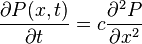
For an equation describing a physical phenomenon, the superposition principle states that a combination of solutions to a linear equation is also a solution of it. When this is true the equation is said to obey the superposition principle. Thus if state vectors $f 1$ , $f 2$ and $f 3$ each solve the linear equation on ψ, then $ψ = c 1 f 1 + c 2 f 2 + c 3 f 3$ would also be a solution, in which each $c$ is a coefficient. The Schroedinger equation is linear, so quantum mechanics follows this.

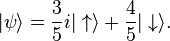
For example, consider an electron with two possible configurations, up and down. This describes the physical system of a qubit.

c_1 \mid \uparrow \rangle + c_2 \mid \downarrow \rangle

is the most general state. But these coefficients dictate probabilities for the system to be in either configuration. The probability for a specified configuration is given by the square of the absolute value of the coefficient. So the probabilities should add up to 1. The electron is in one of those two states for sure.

p_\text{up} = \mid c_1 \mid^2

p_\text{down} = \mid c_2 \mid^2

p_\text{up or down} = p_\text{up} + p_\text{down} = 1

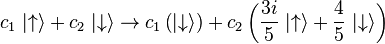
Continuing with this example: If a particle can be in state up and down, it can also be in a state where it is an amount $3 i /5$ in up and an amount $4/5$ in down.

|\psi\rangle = {3\over 5} i |\uparrow\rangle + {4\over 5} |\downarrow\rangle.

In this, the probability for up is $\left|\;\frac{3i}{5}\;\right|^2=\frac{9}{25}$ . The probability for down is $\left|\;\frac{4}{5}\;\right|^2=\frac{16}{25}$ . Note that $\frac{9}{25}+\frac{16}{25}=1$ .

In the description, only the relative size of the different components matter, and their angle to each other on the complex plane. This is usually stated by declaring that two states which are a multiple of one another are the same as far as the description of the situation is concerned. Either of these describe the same state for any nonzero $\alpha$

|\psi \rangle \approx \alpha |\psi \rangle

The fundamental law of quantum mechanics is that the evolution is linear, meaning that if state A turns into A′ and B turns into B′ after 10 seconds, then after 10 seconds the superposition $\psi$ turns into a mixture of A′ and B′ with the same coefficients as A and B.

For example, if we have the following

\mid \uparrow \rangle \to \mid \downarrow \rangle

\mid \downarrow \rangle \to \frac{3i}{5} \mid \uparrow \rangle + \frac{4}{5} \mid \downarrow \rangle

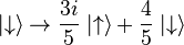
Then after those 10 seconds our state will change to

c_1 \mid \uparrow \rangle + c_2 \mid \downarrow \rangle \to c_1 \left( \mid \downarrow \rangle\right) + c_2 \left(\frac{3i}{5} \mid \uparrow \rangle + \frac{4}{5} \mid \downarrow \rangle \right)

So far there have just been 2 configurations, but there can be infinitely many.

In illustration, a particle can have any position, so that there are different configurations which have any value of the position $x$ . These are written:

|x\rangle

The principle of superposition guarantees that there are states which are arbitrary superpositions of all the positions with complex coefficients:

\sum_x \psi(x) |x\rangle

This sum is defined only if the index $x$ is discrete. If the index is over $\reals$ , then the sum replaced by an integral. The quantity $\psi(x)$ is called the wavefunction of the particle.

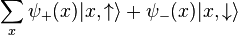
If we consider a qubit with both position and spin, the state is a superposition of all possibilities for both:

\sum_x \psi_+(x)|x,\uparrow\rangle + \psi_-(x)|x,\downarrow\rangle \,

The configuration space of a quantum mechanical system cannot be worked out without some physical knowledge. The input is usually the allowed different classical configurations, but without the duplication of including both position and momentum.

A pair of particles can be in any combination of pairs of positions. A state where one particle is at position x and the other is at position y is written $|x,y\rangle$ . The most general state is a superposition of the possibilities:

\sum_{xy} A(x,y) |x,y\rangle \,

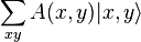
The description of the two particles is much larger than the description of one particle—it is a function in twice the number of dimensions. This is also true in probability, when the statistics of two random variables are correlated. If two particles are uncorrelated, the probability distribution for their joint position $P(x, y)$ is a product of the probability of finding one at one position and the other at the other position:

P(x,y) = P_x (x) P_y(y) \,

In quantum mechanics, two particles can be in special states where the amplitudes of their position are uncorrelated. For quantum amplitudes, the word entanglement replaces the word correlation, but the analogy is exact. A disentangled wave function has the form:

A(x,y) = \psi_x(x)\psi_y(y) \,

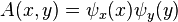
while an entangled wavefunction does not have this form.

Analogy with probability

In probability theory there is a similar principle. If a system has a probabilistic description, this description gives the probability of any configuration, and given any two different configurations, there is a state which is partly this and partly that, with positive real number coefficients, the probabilities, which say how much of each there is.

For example, if we have a probability distribution for where a particle is, it is described by the "state"

\sum_x \rho(x) |x\rangle

Where $\rho$ is the probability density function, a positive number that measures the probability that the particle will be found at a certain location.

The evolution equation is also linear in probability, for fundamental reasons. If the particle has some probability for going from position x to y, and from z to y, the probability of going to y starting from a state which is half-x and half-z is a half-and-half mixture of the probability of going to y from each of the options. This is the principle of linear superposition in probability.

Quantum mechanics is different, because the numbers can be positive or negative. While the complex nature of the numbers is just a doubling, if you consider the real and imaginary parts separately, the sign of the coefficients is important. In probability, two different possible outcomes always add together, so that if there are more options to get to a point z, the probability always goes up. In quantum mechanics, different possibilities can cancel.

In probability theory with a finite number of states, the probabilities can always be multiplied by a positive number to make their sum equal to one. For example, if there is a three state probability system:

x |1\rangle + y |2\rangle + z |3\rangle \,

where the probabilities $x,y,z$ are positive numbers. Rescaling x,y,z so that

x+y+z=1 \,

The geometry of the state space is a revealed to be a triangle. In general it is a simplex. There are special points in a triangle or simplex corresponding to the corners, and these points are those where one of the probabilities is equal to 1 and the others are zero. These are the unique locations where the position is known with certainty.

In a quantum mechanical system with three states, the quantum mechanical wavefunction is a superposition of states again, but this time twice as many quantities with no restriction on the sign:

A|1\rangle + B|2\rangle + C|3\rangle = (A_r + iA_i) |1\rangle + (B_r + i B_i) |2\rangle + (C_r + iC_i) |3\rangle \,

rescaling the variables so that the sum of the squares is 1, the geometry of the space is revealed to be a high-dimensional sphere

A_r^2 + A_i^2 + B_r^2 + B_i^2 + C_r^2 + C_i^2 = 1 \,

A sphere has a large amount of symmetry, it can be viewed in different coordinate systems or bases. So unlike a probability theory, a quantum theory has a large number of different bases in which it can be equally well described. The geometry of the phase space can be viewed as a hint that the quantity in quantum mechanics which corresponds to the probability is the absolute square of the coefficient of the superposition.

Hamiltonian evolution

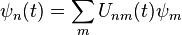
The numbers that describe the amplitudes for different possibilities define the kinematics, the space of different states. The dynamics describes how these numbers change with time. For a particle that can be in any one of infinitely many discrete positions, a particle on a lattice, the superposition principle tells you how to make a state:

\sum_n \psi_n |n\rangle \,

So that the infinite list of amplitudes $\scriptstyle (... \psi_{-2},\psi_{-1},\psi_0,\psi_1,\psi_2 ...)$ completely describes the quantum state of the particle. This list is called the state vector, and formally it is an element of a Hilbert space, an infinite dimensional complex vector space. It is usual to represent the state so that the sum of the absolute squares of the amplitudes add up to one:

\sum \psi_n^*\psi_n = 1

For a particle described by probability theory random walking on a line, the analogous thing is the list of probabilities $(...P_{-2},P_{-1},P_0,P_1,P_2,...)$ , which give the probability of any position. The quantities that describe how they change in time are the transition probabilities $\scriptstyle K_{x\rightarrow y}(t)$ , which gives the probability that, starting at x, the particle ends up at y after time t. The total probability of ending up at y is given by the sum over all the possibilities

P_y(t_0+t) = \sum_x P_x(t_0) K_{x\rightarrow y}(t) \,

The condition of conservation of probability states that starting at any x, the total probability to end up somewhere must add up to 1:

\sum_y K_{x\rightarrow y} = 1 \,

So that the total probability will be preserved, K is what is called a stochastic matrix.

When no time passes, nothing changes: for zero elapsed time $\scriptstyle K{x\rightarrow y}(0) = \delta_{xy}$ , the K matrix is zero except from a state to itself. So in the case that the time is short, it is better to talk about the rate of change of the probability instead of the absolute change in the probability.

P_y(t+dt) = P_y(t) + dt \sum_x P_x R_{x\rightarrow y} \,

where $\scriptstyle R_{x\rightarrow y}$ is the time derivative of the K matrix:

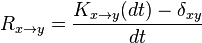
R_{x\rightarrow y} = { K_{x\rightarrow y}(dt) - \delta_{xy} \over dt} \,

The equation for the probabilities is a differential equation which is sometimes called the master equation:

{dP_y \over dt} = \sum_x P_x R_{x\rightarrow y} \,

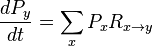
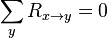
The R matrix is the probability per unit time for the particle to make a transition from x to y. The condition that the K matrix elements add up to one becomes the condition that the R matrix elements add up to zero:

\sum_y R_{x\rightarrow y} = 0 \,

One simple case to study is when the R matrix has an equal probability to go one unit to the left or to the right, describing a particle which has a constant rate of random walking. In this case $\scriptstyle R_{x\rightarrow y}$ is zero unless y is either x+1,x, or x−1, when y is x+1 or x−1, the R matrix has value c, and in order for the sum of the R matrix coefficients to equal zero, the value of $R_{x\rightarrow x}$ must be −2c. So the probabilities obey the discretized diffusion equation:

{dP_x \over dt } = c(P_{x+1} - 2P_{x} + P_{x-1}) \,

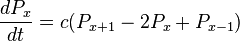
which, when c is scaled appropriately and the P distribution is smooth enough to think of the system in a continuum limit becomes:

{\partial P(x,t) \over \partial t} = c {\partial^2 P \over \partial x^2 } \,

Which is the diffusion equation.

Quantum amplitudes give the rate at which amplitudes change in time, and they are mathematically exactly the same except that they are complex numbers. The analog of the finite time K matrix is called the U matrix:

\psi_n(t) = \sum_m U_{nm}(t) \psi_m \,

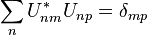
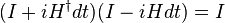
Since the sum of the absolute squares of the amplitudes must be constant, $U$ must be unitary:

\sum_n U^*_{nm} U_{np} = \delta_{mp} \,

or, in matrix notation,

U^\dagger U = I \,

The rate of change of U is called the Hamiltonian H, up to a traditional factor of i:

H_{mn} = i{d \over dt} U_{mn}

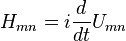
The Hamiltonian gives the rate at which the particle has an amplitude to go from m to n. The reason it is multiplied by i is that the condition that U is unitary translates to the condition:

(I + i H^\dagger dt )(I - i H dt ) = I \,

H^\dagger - H = 0 \,

which says that H is Hermitian. The eigenvalues of the Hermitian matrix H are real quantities which have a physical interpretation as energy levels. If the factor i were absent, the H matrix would be antihermitian and would have purely imaginary eigenvalues, which is not the traditional way quantum mechanics represents observable quantities like the energy.

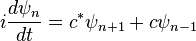
For a particle which has equal amplitude to move left and right, the Hermitian matrix H is zero except for nearest neighbors, where it has the value c. If the coefficient is everywhere constant, the condition that H is Hermitian demands that the amplitude to move to the left is the complex conjugate of the amplitude to move to the right. The equation of motion for $\psi$ is the time differential equation:

i{d \psi_n \over dt} = c^* \psi_{n+1} + c \psi_{n-1}

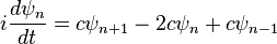
In the case that left and right are symmetric, c is real. By redefining the phase of the wavefunction in time, $\psi\rightarrow \psi e^{i2ct}$ , the amplitudes for being at different locations are only rescaled, so that the physical situation is unchanged. But this phase rotation introduces a linear term.

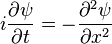
i{d \psi_n \over dt} = c \psi_{n+1} - 2c\psi_n + c\psi_{n-1}

which is the right choice of phase to take the continuum limit. When c is very large and psi is slowly varying so that the lattice can be thought of as a line, this becomes the free Schrödinger equation:

i{ \partial \psi \over \partial t } = - {\partial^2 \psi \over \partial x^2}

If there is an additional term in the H matrix which is an extra phase rotation which varies from point to point, the continuum limit is the Schrödinger equation with a potential energy:

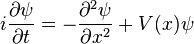
i{ \partial \psi \over \partial t} = - {\partial^2 \psi \over \partial x^2} + V(x) \psi

These equations describe the motion of a single particle in non-relativistic quantum mechanics.

Quantum mechanics in imaginary time

The analogy between quantum mechanics and probability is very strong, so that there are many mathematical links between them. In a statistical system in discrete time, t=1,2,3, described by a transition matrix for one time step $\scriptstyle K_{m\rightarrow n}$ , the probability to go between two points after a finite number of time steps can be represented as a sum over all paths of the probability of taking each path:

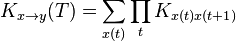
K_{x\rightarrow y}(T) = \sum_{x(t)} \prod_t K_{x(t)x(t+1)} \,

where the sum extends over all paths $x(t)$ with the property that $x(0)=0$ and $x(T)=y$ . The analogous expression in quantum mechanics is the path integral.

A generic transition matrix in probability has a stationary distribution, which is the eventual probability to be found at any point no matter what the starting point. If there is a nonzero probability for any two paths to reach the same point at the same time, this stationary distribution does not depend on the initial conditions. In probability theory, the probability m for the stochastic matrix obeys detailed balance when the stationary distribution $\rho_n$ has the property:

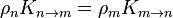
\rho_n K_{n\rightarrow m} = \rho_m K_{m\rightarrow n} \,

Detailed balance says that the total probability of going from m to n in the stationary distribution, which is the probability of starting at m $\rho_m$ times the probability of hopping from m to n, is equal to the probability of going from n to m, so that the total back-and-forth flow of probability in equilibrium is zero along any hop. The condition is automatically satisfied when n=m, so it has the same form when written as a condition for the transition-probability R matrix.

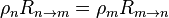
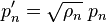
\rho_n R_{n\rightarrow m} = \rho_m R_{m\rightarrow n} \,

When the R matrix obeys detailed balance, the scale of the probabilities can be redefined using the stationary distribution so that they no longer sum to 1:

p'_n = \sqrt{\rho_n}\;p_n \,

In the new coordinates, the R matrix is rescaled as follows:

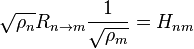
\sqrt{\rho_n} R_{n\rightarrow m} {1\over \sqrt{\rho_m}} = H_{nm} \,

and H is symmetric

H_{nm} = H_{mn} \,

This matrix H defines a quantum mechanical system:

i{d \over dt} \psi_n = \sum H_{nm} \psi_m \,

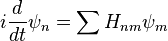
whose Hamiltonian has the same eigenvalues as those of the R matrix of the statistical system. The eigenvectors are the same too, except expressed in the rescaled basis. The stationary distribution of the statistical system is the ground state of the Hamiltonian and it has energy exactly zero, while all the other energies are positive. If H is exponentiated to find the U matrix:

U(t) = e^{-iHt} \,

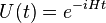
and t is allowed to take on complex values, the K' matrix is found by taking time imaginary.

K'(t) = e^{-Ht} \,

For quantum systems which are invariant under time reversal the Hamiltonian can be made real and symmetric, so that the action of time-reversal on the wave-function is just complex conjugation. If such a Hamiltonian has a unique lowest energy state with a positive real wave-function, as it often does for physical reasons, it is connected to a stochastic system in imaginary time. This relationship between stochastic systems and quantum systems sheds much light on supersymmetry.

Experiments and applications

Successful experiments involving superpositions of relatively large (by the standards of quantum physics) objects have been performed.^[18]

A "cat state" has been achieved with photons.^[19]
A beryllium ion has been trapped in a superposed state.^[20]
A double slit experiment has been performed with molecules as large as buckyballs.^[21]^[22]
An experiment involving a superconducting quantum interference device ("SQUID") has been linked to theme of the "cat state" thought experiment.^[23]

By use of very low temperatures, very fine experimental arrangements were made to protect in near isolation and preserve the coherence of intermediate states, for a duration of time, between preparation and detection, of SQUID currents. Such a SQUID current is a coherent physical assembly of perhaps billions of electrons. Because of its coherence, such an assembly may be regarded as exhibiting "collective states" of a macroscopic quantal entity. For the principle of superposition, after it is prepared but before it is detected, it may be regarded as exhibiting an intermediate state. It is not a single-particle state such as is often considered in discussions of interference, for example by Dirac in his famous dictum stated above.^[24] Morever, though the 'intermediate' state may be loosely regarded as such, it has not been produced as an output of a secondary quantum analyser that was fed a pure state from a primary analyser, and so this is not an example of superposition as strictly and narrowly defined.

Nevertheless, after preparation, but before measurement, such a SQUID state may be regarded in a manner of speaking as a "pure" state that is a superposition of a clockwise and an anti-clockwise current state. In a SQUID, collective electron states can be physically prepared in near isolation, at very low temperatures, so as to result in protected coherent intermediate states. Remarkable here is that there are found two well-separated respectively self-coherent collective states that exhibit such metastability. The crowd of electrons tunnels back and forth between the clockwise and the anti-clockwise states, as opposed to forming a single intermediate state in which there is no definite collective sense of current flow.^[25]^[26]

In contrast, for actual real cats, such well-separated metastable collective states states do not exist and consequently cannot be physically prepared. Schrödinger's point was that classical thinking does not in general anticipate such physically distinct and separate metastable quantum states. In classical thinking, distinct quantum states even of single atoms can indeed be regarded as metastable, and are remarkable and unexpected. In the days when Schrödinger raised his argumentative example, no one had imagined the invention of SQUIDs that exhibit such states on a macroscopic scale. The present-day physicist here pays close attention to the requirement mentioned above, that the intermediate states must be carefully physically shielded to protect them from any factor that affects some of the independent quantal entities (in this case collective not single particle) differently from others. Contrary to this requirement, the living cat breathes. This destroys intermediate state coherence, and so the conditions required for exhibition of the principle of superposition are not fulfilled.

A piezoelectric "tuning fork" has been constructed, which can be placed into a superposition of vibrating and non vibrating states. The resonator comprises about 10 trillion atoms.^[27]
Recent research indicates that chlorophyll within plants appears to exploit the feature of quantum superposition to achieve greater efficiency in transporting energy, allowing pigment proteins to be spaced further apart than would otherwise be possible.^[28]^[29]

In quantum computing the phrase "cat state" often refers to the special entanglement of qubits wherein the qubits are in an equal superposition of all being 0 and all being 1; i.e.,

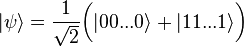| \psi \rangle = \frac{1}{\sqrt{2}} \bigg( | 00...0 \rangle + |11...1 \rangle \bigg)

Formal interpretation

Applying the superposition principle to a quantum mechanical particle, the configurations of the particle are all positions, so the superpositions make a complex wave in space. The coefficients of the linear superposition are a wave which describes the particle as best as is possible, and whose amplitude interferes according to the Huygens principle.

For any physical property in quantum mechanics, there is a list of all the states where that property has some value. These states are necessarily perpendicular to each other using the Euclidean notion of perpendicularity which comes from sums-of-squares length, except that they also must not be i multiples of each other. This list of perpendicular states has an associated value which is the value of the physical property. The superposition principle guarantees that any state can be written as a combination of states of this form with complex coefficients.

Write each state with the value q of the physical quantity as a vector in some basis $\psi^q_n$ , a list of numbers at each value of n for the vector which has value q for the physical quantity. Now form the outer product of the vectors by multiplying all the vector components and add them with coefficients to make the matrix

A_{nm} = \sum_q q \psi^{*q}_n \psi^q_m

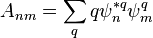
where the sum extends over all possible values of q. This matrix is necessarily symmetric because it is formed from the orthogonal states, and has eigenvalues q. The matrix A is called the observable associated to the physical quantity. It has the property that the eigenvalues and eigenvectors determine the physical quantity and the states which have definite values for this quantity.

Every physical quantity has a Hermitian linear operator associated to it, and the states where the value of this physical quantity is definite are the eigenstates of this linear operator. The linear combination of two or more eigenstates results in quantum superposition of two or more values of the quantity. If the quantity is measured, the value of the physical quantity will be random, with a probability equal to the square of the coefficient of the superposition in the linear combination. Immediately after the measurement, the state will be given by the eigenvector corresponding to the measured eigenvalue.

Physical interpretation

It is natural to ask why ordinary everyday "real" (macroscopic, Newtonian) objects and events do not seem empirically to display quantum mechanical features such as superposition. Indeed, this is sometimes regarded even as "mysterious", for example by Richard Feynman.^[30] In 1935, Erwin Schrödinger devised a well-known thought experiment, now known as Schrödinger's cat, which highlighted the dissonance between quantum mechanics and Newtonian physics, where only one configuration occurs, although a configuration for a particle in Newtonian physics specifies both position and momentum.

The explanation is as follows. It is a logical truism that a single detection of a quantal entity, observed alone, empirically considered, is not an example of a relation of several states. For the several states are not empirically defined when the quantal entity is observed alone. It would therefore be nonsense to try to say that it, a single state, observed alone, empirically shows superposition. Superposition is a relation of several states that are empirically defined only when several intermediate beams are empirically verified to be present. Actual empirical observation of superposition requires that the several intermediate beams should be actually observed, in several distinct experimental set-ups. Without the several experiments, talk of superposition is mere theoretical speculation, not empirical observation. The superposed state is, as defined above, also a pure state, with respect to the primary analyser. It is classically inexplicable how a quantum analyser can have several pure states as outputs. That is Feynman's "mystery".

Quantum superposition is exhibited in fact in many directly observable phenomena, such as interference peaks from an electron wave in a double-slit experiment. Superposition persists at all scales, provided that coherence is shielded from disruption by intermittent external factors. This is a reason for differences of opinion, as between the Copenhagen or other interpretations.

The Heisenberg uncertainty principle states that for any given instant of time, the position and velocity of an electron or other subatomic particle cannot both be exactly determined.

If the operators corresponding to two observables do not commute, they have no simultaneous eigenstates and they obey the uncertainty principle. A state where one observable has a definite value corresponds to a superposition of many states for the other observable.

References

↑ Dirac, P.A.M. (1958), pp. 11–12.
↑
- Messiah, A. (1961), p. 197, 199.
↑ Cohen-Tannoudji, C., Diu, B., Laloë, F. (1973/1977), p. 260.
↑
- Messiah, A. (1961), p. 204–205.
↑ 5.0 5.1 Feynman, R.P., Leighton, R.B., Sands, M. (1965), Chapter 6.
↑ Merzbacher, E. (1961/1970), p. 219.
↑ Bartell, L.S. (1980). Complementarity in the double-slit experiment: on simple realizable systems for observing intermediate particle-wave behavior, Phys. Rev. D 21: 1698–1699.
↑ Aspect, A., Dalibard, J., Roger, G. (1982). Experimental tests of Bell's inequalities using time-varying analysers, Phys. Rev. Lett. 49: 1804–1807.
↑ McIntyre, D.H. (2012). Quantum Mechanics: a Paradigms Approach, Pearson Addison-Wesley, San Francisco, ISBN 978-0-321-76579-6, Chapter 1.
↑ Dirac, P.A.M. (1958), pp. 12–13.
↑ Bohr, N. (1927/1928), p. 580.
↑ Feynman, R.P., Leighton, R.B., Sands, M. (1965), Chapter 5.
↑ Dirac P.A.M. (1930/1958), p. 12.
↑ Bacciagaluppi, G. (2012). The role of decoherence in quantum mechanics.
↑ Einstein, A. (1949), p. 670.
↑ Ludwig, G. (1985). An Axiomatic Basis for Quantum Mechanics, vol. 1, Derivation of Hilbert Space Structure, translated from German by L.F. Boron, Springer, Berlin, ISBN 978-3-642-70029-3, passim.
↑ Wheeler, J.A., Zurek, W.H. (1983), pp. viii, xvi, 3, 7, 46, 185, 194, 196.
↑ What is the World's Biggest Schrodinger Cat?
↑ Schrödinger's Cat Now Made of Light
↑ C. Monroe, et. al. A "Schrodinger Cat" Superposition State of an Atom
↑ Wave Particle Duality of C60
↑ Diffraction of the Fullerenes C60 and C70 by a standing light wave
↑ Leggett, A.J. (1986). The superposition principle in macroscopic systems, pp. 28–40 in Quantum Concepts of Space and Time, edited by R. Penrose and C.J. Isham, ISBN 0-19-851972-9.
↑ Dirac, P.A.M. (1930/1958), p. 9.
↑ Physics World: Schrodinger's cat comes into view
↑ Friedman, J.R., Patel, V., Chen, W., Tolpygo, S.K., Lukens, J.E. (2000).Quantum superposition of distinct macroscopic states, Nature 406: 43–46.
↑ Scientific American : Macro-Weirdness: "Quantum Microphone" Puts Naked-Eye Object in 2 Places at Once: A new device tests the limits of Schrödinger's cat
↑ Scholes, Gregory; Elisabetta Collini, Cathy Y. Wong, Krystyna E. Wilk, Paul M. G. Curmi, Paul Brumer & Gregory D. Scholes (4 February 2010). "Coherently wired light-harvesting in photosynthetic marine algae at ambient temperature". Nature 463 (7281): 644–647. Bibcode:2010Natur.463..644C. doi:10.1038/nature08811. PMID 20130647.
↑ Moyer, Michael (September 2009). "Quantum Entanglement, Photosynthesis and Better Solar Cells". Scientific American. Retrieved 12 May 2010.
↑ Feynman, R.P., Leighton, R.B., Sands, M. (1965), § 1-1.

Bibliography of cited references

Bohr, N. (1927/1928). The quantum postulate and the recent development of atomic theory, Nature Supplement April 14 1928, 121: 580–590.
Einstein, A. (1949). Remarks concerning the essays brought together in this co-operative volume, translated from the original German by the editor, pp. 665–688 in Schilpp, P.A. editor (1949), Albert Einstein: Philosopher-Scientist, volume $II$ , Open Court, La Salle IL.
Cohen-Tannoudji, C., Diu, B., Laloë, F. (1973/1977). Quantum Mechanics, translated from the French by S.R. Hemley, N. Ostrowsky, D. Ostrowsky, second edition, volume 1, Wiley, New York, ISBN 0471164321.
Dirac, P.A.M. (1930/1958). The Principles of Quantum Mechanics, 4th edition, Oxford University Press.
Feynman, R.P., Leighton, R.B., Sands, M. (1965). The Feynman Lectures on Physics, volume 3, Addison–Wesley, Reading, MA.

Merzbacher, E. (1961/1970). Quantum Mechanics, second edition, Wiley, New York.
Messiah, A. (1961). Quantum Mechanics, volume 1, translated by G.M. Temmer from the French Mécanique Quantique, North-Holland, Amsterdam.
Wheeler, J.A.; Zurek, W.H. (1983). Quantum Theory and Measurement. Princeton NJ: Princeton University Press.