Quantum pendulum

The quantum pendulum is fundamental in understanding hindered internal rotations in chemistry, quantum features of scattering atoms as well as numerous other quantum phenomena. Though a pendulum not subject to the small-angle approximation has an inherent non-linearity, the Schrödinger equation for the quantized system can be solved relatively easily.

Schrödinger Equation

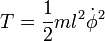
Using Lagrangian theory from classical mechanics, one can develop a Hamiltonian for the system. A simple pendulum has one generalized coordinate (the angular displacement $\phi$ ) and two constraints (the length of the string is constant and there is no motion along the z axis). The kinetic energy and potential energy of the system can be found to be as follows:

T=\frac{1}{2} m l^2 \dot{\phi}^2

U=m g l (1-\cos(\phi))

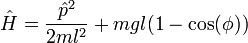
This results in the Hamiltonian:

\hat{H} = \frac{\hat{p}^2}{2 m l^2} + m g l (1-\cos(\phi))

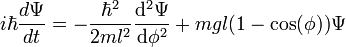
The time-dependent Schrödinger equation for the system is as follows:

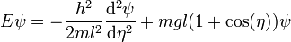
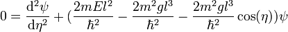
i \hbar \frac{d\Psi}{dt} = - \frac{\hbar^2}{2 m l^2} \frac {\mathrm{d}^2 \Psi} {\mathrm{d} \phi^2}+m g l (1-\cos(\phi)) \Psi

One must solve the time-independent Schrödinger equation to find the energy levels and corresponding eigenstates. This is best accomplished by changing the independent variable as follows:

\eta = \phi + \pi

E \psi = - \frac{\hbar^2}{2 m l^2} \frac {\mathrm{d}^2 \psi} {\mathrm{d} \eta^2}+m g l (1+\cos(\eta)) \psi

This is simply Mathieu's equation where the solutions are Mathieu functions

0 = \frac {\mathrm{d}^2 \psi} {\mathrm{d} \eta^2}+(\frac{2 m E l^2} {\hbar^2}-\frac{2 m^2 g l^3} {\hbar^2}-\frac{2 m^2 g l^3} {\hbar^2} \cos(\eta)) \psi

Solutions

Energies

Given $q$ , for countably many special values of $a$ , called characteristic values, the Mathieu equation admits solutions which are periodic with period $2\pi$ . The characteristic values of the Mathieu cosine, sine functions respectively are written $a_n(q), \, b_n(q)$ , where n is a natural number. The periodic special cases of the Mathieu cosine and sine functions are often written $CE(n,q,x), \, SE(n,q,x)$ respectively, although they are traditionally given a different normalization (namely, that their L² norm equal $\pi$ ).

The boundary conditions in the quantum pendulum imply that $a_n(q), \, b_n(q)$ are as follows for a given q:

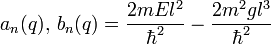
0 = \frac {\mathrm{d}^2 \psi} {\mathrm{d} \eta^2}+(\frac{2 m E l^2} {\hbar^2}-\frac{2 m^2 g l^3} {\hbar^2}-\frac{2 m^2 g l^3} {\hbar^2} \cos(\eta)) \psi

a_n(q), \, b_n(q)=\frac{2 m E l^2} {\hbar^2}-\frac{2 m^2 g l^3} {\hbar^2}

The energies of the system, 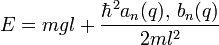$E=m g l+\frac{\hbar^2 a_n(q), \, b_n(q)}{2 m l^2}$ for even/odd solutions respectively, are quantized based on the characteristic values found by solving the Mathieu equation

The effective potential depth can be defined as follows:

$q=\frac{m^2 g l^3} {\hbar^2}$

A depth potential depth yields the dynamics of a particle in an independent potential. In contrast, a shallow potential depth, Bloch waves as well as quantum tunneling become of importance.

General Solution

The general solution of the above differential equation for a given value of a and q is a set of linearly independent Mathieu cosines and Mathieu sines, which are even and odd solutions respectively. In general, the Mathieu functions are aperiodic; however, for characteristic values of $a_n(q), \, b_n(q)$ , the Mathieu cosine and sine become periodic with a period of $2 \pi$ .

Eigenstates

For positive values of q, the following is true:

C \left( a_n(q),q,x \right) = \frac{CE(n,q,x)}{CE(n,q,0)}

S \left( b_n(q),q,x \right) = \frac{SE(n,q,x)}{SE^\prime(n,q,0)}.

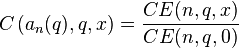
Here are the first few periodic Mathieu cosine functions for q=1:

Note that, for example, $CE(1,1,x)$ (green) resembles a cosine function, but with flatter hills and shallower valleys.

Bibliography

Bransden, B. H.; Joachain, C. J. (2000). Quantum mechanics (2nd ed.). Essex: Pearson Education. ISBN 0-582-35691-1.
Davies, John H. (2006). The Physics of Low-Dimensional Semiconductors: An Introduction (6th reprint ed.). Cambridge University Press. ISBN 0-521-48491-X.
Griffiths, David J. (2004). Introduction to Quantum Mechanics (2nd ed.). Prentice Hall. ISBN 0-13-111892-7.
Muhammad Ayub, Atom Optics Quantum Pendulum, 2011, Islamabad, Pakistan., http://lanl.arxiv.org/PS_cache/arxiv/pdf/1012/1012.6011v1.pdf

External links

Atom Optics Quantum Pendulum