Quantum calculus
Quantum calculus, sometimes called calculus without limits, is equivalent to traditional infinitesimal calculus without the notion of limits. It defines "q-calculus" and "h-calculus". h ostensibly stands for Planck's constant while q stands for quantum. The two parameters are related by the formula
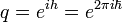
where  is the reduced Planck constant.
Differentiation
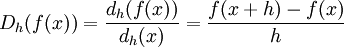
In the q-calculus and h-calculus, differentials of functions are defined as

and

respectively. Derivatives of functions are then defined as fractions by the q-derivative

and by
In the limit, as h goes to 0, or equivalently as q goes to 1, these expressions take on the form of the derivative of classical calculus.
Integration
q-integral
A function F(x) is a q-antiderivative of f(x) if DqF(x)=f(x). The q-antiderivative (or q-integral) is denoted by  and an expression for F(x) can be found from the formula
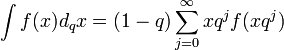 which is called the Jackson integral of f(x). For 0 < q < 1, the series converges to a function F(x) on an interval (0,A] if |f(x)x^α| is bounded on the interval (0,A] for some 0 <= α < 1.
The q-integral is a Riemann-Stieltjes integral with respect to a step function having infinitely many points of increase at the points qj, with the jump at the point qj being qj. If we call this step function gq(t) then dgq(t) = dqt.[1]
h-integral
A function F(x) is an h-antiderivative of f(x) if DhF(x)=f(x). The h-antiderivative (or h-integral) is denoted by  . If a and b differ by an integer multiple of h then the definite integral
 is given by a Riemann sum of f(x) on the interval [a,b] partitioned into subintervals of width h.
Example
The derivative of the function  (for some positive integer
  ) in the classical calculus is
  . The corresponding expressions in q-calculus and h-calculus are
![D_q(x^n) = \frac{q^n - 1}{q - 1} x^{n - 1} = [n]_q\ x^{n - 1}](../I/m/13c767659b3d32b645f0c23e419b0e99.png)
with the q-bracket
![[n]_q = \frac{q^n - 1}{q - 1}](../I/m/8a8ec4d1f60a5190fafef69a59629a92.png)
and

respectively. The expression ![[n]_q x^{n - 1}](../I/m/4d8d0cb7d38d936c90b4df4217b837fa.png) is then the q-calculus analogue of the simple power rule for
positive integral powers. In this sense, the function is still nice in the q-calculus, but rather
ugly in the h-calculus – the h-calculus analog of is instead the falling factorial,
is then the q-calculus analogue of the simple power rule for
positive integral powers. In this sense, the function is still nice in the q-calculus, but rather
ugly in the h-calculus – the h-calculus analog of is instead the falling factorial,  One may proceed further and develop, for example, equivalent notions of Taylor expansion, et cetera, and even arrive at q-calculus analogues for all of the usual functions one would want to have, such as an analogue for the sine function whose q-derivative is the appropriate analogue for the cosine.
History
The h-calculus is just the calculus of finite differences, which had been studied by George Boole and others, and has proven useful in a number of fields, among them combinatorics and fluid mechanics. The q-calculus, while dating in a sense back to Leonhard Euler and Carl Gustav Jacobi, is only recently beginning to see more usefulness in quantum mechanics, having an intimate connection with commutativity relations and Lie algebra.
See also
- Noncommutative geometry
- Quantum differential calculus
- Time scale calculus
- q-analog
References
- ↑ FUNCTIONS q-ORTHOGONAL WITH RESPECT TO THEIR OWN ZEROS, LUIS DANIEL ABREU, Pre-Publicacoes do Departamento de Matematica Universidade de Coimbra, Preprint Number 04–32
- F. H. Jackson (1908), "On q-functions and a certain difference operator", Trans. Roy. Soc. Edin., 46 253-281.
- Exton, H. (1983), q-Hypergeometric Functions and Applications, New York: Halstead Press, Chichester: Ellis Horwood, 1983, ISBN 0853124914, ISBN 0470274530, ISBN 978-0470274538
- Victor Kac, Pokman Cheung, Quantum calculus, Universitext, Springer-Verlag, 2002. ISBN 0-387-95341-8