Proximal gradient method
Proximal gradient methods are a generalized form of projection used to solve non-differentiable convex optimization problems. Many interesting problems can be formulated as convex optimization problems of form

where  are convex functions defined from
 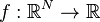 where some of the functions are non-differentiable, this rules out our conventional smooth optimization techniques like
Steepest descent method, conjugate gradient method etc. There is a specific class of algorithms which can solve above optimization problem. These methods proceed by splitting,
in that the functions
where some of the functions are non-differentiable, this rules out our conventional smooth optimization techniques like
Steepest descent method, conjugate gradient method etc. There is a specific class of algorithms which can solve above optimization problem. These methods proceed by splitting,
in that the functions  are used individually so as to yield an easily implementable algorithm.
They are called proximal because each non smooth function among is involved via its proximity
operator. Iterative Shrinkage thresholding algorithm, projected Landweber, projected
gradient, alternating projections, alternating-direction method of multipliers, alternating
split Bregman are special instances of proximal algorithms. Details of proximal methods are discussed in Combettes and Pesquet.[1] For the theory of proximal gradient methods from the perspective of and with applications to statistical learning theory, see proximal gradient methods for learning.
are used individually so as to yield an easily implementable algorithm.
They are called proximal because each non smooth function among is involved via its proximity
operator. Iterative Shrinkage thresholding algorithm, projected Landweber, projected
gradient, alternating projections, alternating-direction method of multipliers, alternating
split Bregman are special instances of proximal algorithms. Details of proximal methods are discussed in Combettes and Pesquet.[1] For the theory of proximal gradient methods from the perspective of and with applications to statistical learning theory, see proximal gradient methods for learning.
Notations and terminology
Let  , the
, the  -dimensional euclidean space, be the domain of the function
![f: \mathbb{R}^N \rightarrow [-\infty,+\infty]](../I/m/bab8497226fb81a846113b0652e1e3a1.png) . Suppose
. Suppose  is the non-empty
convex subset of . Then, the indicator function of is defined as
is the non-empty
convex subset of . Then, the indicator function of is defined as
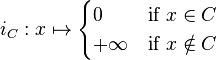
-
 -norm is defined as (
  )
)

The distance from  to is defined as
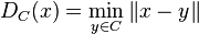
If is closed and convex, the projection of onto is the unique point
 such that
  .
.
The subdifferential of  is given by

Projection onto convex sets (POCS)
One of the widely used convex optimization algorithms is POCS (Projection Onto Convex Sets).
This algorithm is employed to recover/synthesize a signal satisfying simultaneously several convex constraints.
Let  be the indicator function of non-empty closed convex set
  modeling a constraint.
This reduces to convex feasibility problem, which require us to find a solution such that it lies in the intersection
of all convex sets . In POCS method each set is incorporated by its projection operator
modeling a constraint.
This reduces to convex feasibility problem, which require us to find a solution such that it lies in the intersection
of all convex sets . In POCS method each set is incorporated by its projection operator
 . So in each iteration
  is updated as

However beyond such problems projection operators are not appropriate and more general operators are required to tackle them. Among the various generalizations of the notion of a convex projection operator that exist, proximity operators are best suited for other purposes.
Definition
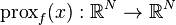
Proximity operators of function at is defined as
For every , the minimization problem
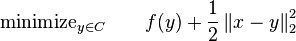
admits a unique solution which is denoted by  .
.
The proximity operator of is characterized by inclusion

If is differentiable then above equation reduces to

Examples
Special instances of Proximal Gradient Methods are
- Projected Landweber
- Alternating projection
- Alternating-direction method of multipliers
- Fast Iterative Shrinkage Thresholding Algorithm (FISTA)[2]
See also
- Alternating projection
- Convex optimization
- Frank–Wolfe algorithm
- Proximal gradient methods for learning
References
- Rockafellar, R. T. (1970). Convex analysis. Princeton: Princeton University Press.
- Combettes, Patrick L.; Pesquet, Jean-Christophe (2011). Springer's Fixed-Point Algorithms for Inverse Problems in Science and Engineering 49. pp. 185–212.
Notes
- ↑ Combettes, Patrick L.; Pesquet, Jean-Christophe (2009). "Proximal Splitting Methods in Signal Processing". p. {11–23}.
- ↑ "Beck, A; Teboulle, M (2009). "A fast iterative shrinkage-thresholding algorithm for linear inverse problems". SIAM J. Imaging Science 2. pp. 183–202.
External links
- Stephen Boyd and Lieven Vandenberghe Book, Convex optimization
- EE364a: Convex Optimization I and EE364b: Convex Optimization II, Stanford course homepages
- EE227A: Lieven Vandenberghe Notes Lecture 18