Preisach model of hysteresis

The Preisach model of hysteresis generalizes hysteresis loops as the parallel connection of independent relay hysterons. It was first suggested in 1935 by Ferenc (Franz) Preisach^[1] in the German academic journal "Zeitschrift für Physik".^[2] Since then, it has become a widely accepted model of hysteresis.^[3] The Preisach model is especially accurate in the field of ferromagnetism, as the ferromagnetic material can be described as a network of small domains, each magnetized to a value of either $h$ or $-h$ . A sample of iron, for example, may have randomly distributed magnetic domains, resulting in a net magnetic field of zero.

Nonideal relay

The relay hysteron is the fundamental building block of the Preisach model. It is described as a two-valued operator denoted by $R_{\alpha,\beta}$ . Its I/O map takes the form of a loop, as shown:

Above, a relay of magnitude 1. $\alpha$ defines the "switch-off" threshold, and $\beta$ defines the "switch-on" threshold.

Graphically, if $x$ is less than $\alpha$ , the output $y$ is "low" or "off." As we increase $x$ , the output remains low until $x$ reaches $\beta$ —at which point the output switches "on." Further increasing $x$ has no change. Decreasing $x$ , $y$ does not go low until $x$ reaches $\alpha$ again. It is apparent that the relay operator $R_{\alpha,\beta}$ takes the path of a loop, and its next state depends on its past state.

Mathematically, the output of $R_{\alpha,\beta}$ is expressed as:

$y(x)=\begin{cases} 1&\mbox{ if }x\geq\beta\\ 0&\mbox{ if }x\leq\alpha \\ k&\mbox{ if }\alpha<x<\beta \end{cases}$

Where $k=0$ if the last time $x$ was outside of the boundaries $\alpha<x<\beta$ , it was in the region of $x\leq\alpha$ ; and $k=1$ if the last time $x$ was outside of the boundaries $\alpha<x<\beta$ , it was in the region of $x\geq\beta$ .

This definition of the hysteron shows that the current value $y$ of the complete hysteresis loop depends upon the history of the input variable $x$ .

Discrete Preisach model

The Preisach Model consists of many relay hysterons connected in parallel, given weights, and summed. This is best visualized by a block diagram:

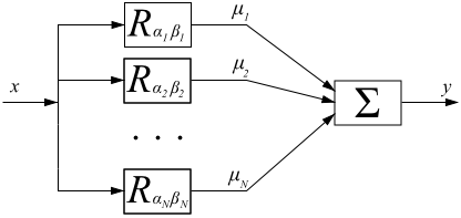
Each of these relays has different $\alpha$ and $\beta$ thresholds and is scaled by $\mu$ . Each relay can be plotted on a so-called Preisach plane with its $(\alpha,\beta)$ values. Depending on their distribution on the Preisach plane, the relay hysterons can represent hysteresis with good accuracy. As well, with increasing $N$ , the true hysteresis curve is approximated better.

In the limit as $N$ approaches infinity, we obtain the continuous Preisach model.

The $\alpha\beta$ plane

One of the easiest ways to look at the preisach model is using a geometric interpretation. Consider a plane of coordinates $\alpha\beta$ . On this plane, each point $(\alpha_{i},\beta_{i})$ is mapped to a specific relay hysteron $R_{\alpha_{i},\beta_{i}}$ .

We consider only the half-plane $\alpha<\beta$ as any other case does not have a physical equivalent in nature.

Next, we take a specific point on the half plane and build a right triangle by drawing two lines parallel to the axes, both from the point to the line $\alpha=\beta$ .

We now present the Preisach density function, denoted $\mu(\alpha,\beta)$ . This function describes the amount of relay hysterons of each distinct values of $(\alpha_{i},\beta_{i})$ . As a default we say that outside the right triangle $\mu(\alpha,\beta)=0$ .

A modified formulation of the classical Preisach model has been presented, allowing analitycal expression of the Everett function.^[4] This makes the model considerably faster and especially adequate for inclusion in electromagnetic field computation or electric circuit analysis codes.

References

↑ Ralph Smith, Smart material systems: model development, SIAM, 2005. p. 189.
↑ F. Preisach, Über die magnetische Nachwirkung. Zeitschrift für Physik, 94:277-302, 1935
↑ Augusto Visintin, Differential Models of Hysteresis (Applied Mathematical Sciences), Springer, 1995
↑ Zs. Szabó, “Preisach Functions Leading to Closed Form Permeability“, Physica B, vol. 372, pp. 61-67, 2006.

External links