Poynting vector

| Electromagnetism |
|---|
 |
In physics, the Poynting vector represents the directional energy flux density (the rate of energy transfer per unit area) of an electromagnetic field. The SI unit of the Poynting vector is the watt per square metre (W/m2). It is named after its inventor John Henry Poynting. Oliver Heaviside[1] and Nikolay Umov independently co-invented the Poynting vector.
Definition
In Poynting's original paper and in many textbooks, it is usually denoted by S or N, and defined as (all bold letters represent vectors)[2][3]

where
- E is the electric field;
- H is the magnetic field.
This form is often called the Abraham form.[4][5] Occasionally an alternative definition in terms of electric field E and magnetic flux density B is used. It is even possible to combine the electric displacement field D with the magnetic flux density B to get the Minkowski form of the Poynting vector, or use D and H to construct another.[6] The choice has been controversial: Pfeifer et al.[7] summarize and to a certain extent resolve the century-long dispute between proponents of the Abraham and Minkowski forms.
The Poynting vector represents the particular case of an energy flux vector for electromagnetic energy. However, any type of energy has its direction of movement in space, as well as its density, so energy flux vectors can be defined for other types of energy as well, e.g., for mechanical energy. The Umov–Poynting vector[8] discovered by Nikolay Umov in 1874 describes energy flux in liquid and elastic media in a completely generalized view.
Interpretation

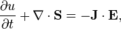
The Poynting vector appears in Poynting's theorem (see this article for the derivation of the theorem and vector), an energy-conservation law:[5]
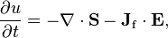
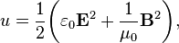
where Jf is the current density of free charges and u is the electromagnetic energy density, given by
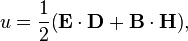
where
- E is the electric field;
- D is the electric displacement field;
- B is the magnetic flux density;
- H is the magnetic field.
The first term in the right-hand side represents the net electromagnetic energy flow into a small volume, while the second term represents the subtracted portion of the work done by free electrical currents that are not necessarily converted into electromagnetic energy (dissipation, heat). In this definition, bound electrical currents are not included in this term, and instead contribute to S and u.
Note that u can only be given if linear, nondispersive and uniform materials are involved, i.e., if the constitutive relations can be written as
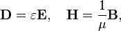
where
- ε is the permittivity of the material;
- μ is the permeability of the material.[5]
In principle, this limits Poynting's theorem in this form to fields in vacuum. A generalization to dispersive materials is possible under certain circumstances at the cost of additional terms and the loss of their clear physical interpretation.[5]
The Poynting vector is usually interpreted as an energy flux, but this is only strictly correct for electromagnetic radiation. The more general case is described by Poynting's theorem above, where it occurs as a divergence, which means that it can only describe the change of energy density in space, rather than the flow.
Invariance to adding a curl of a field
Since the Poynting vector only occurs in Poynting's theorem as a divergence ∇ ⋅ S, the Poynting vector S is arbitrary to the extent that one can add a curl of a field F to S:[5]

since the divergence of the curl term is zero: ∇ ⋅ (∇ × F) = 0 for an arbitrary field F (see Vector calculus identities).
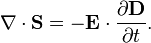
This property is used in quasi-electrostatic regimes to describe for instance energy propagating through waves in piezoelectric materials. In such cases magnetic fields are negligible and a local flux of energy can be defined based on electrical quantities only. In the general case we can express the divergence of the Poynting vector as

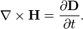
The fourth of the Maxwell's equations writes
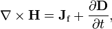
where Jf is the current density due to free charges.
In dielectric materials it reduces to
Combining the two previous results, leads to the following quasi-electrostatic divergence:
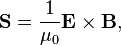
A new "magnetic free" Poynting vector leading to the same divergence can be defined as
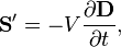
where V is the electrostatic potential.
A demonstration in the case of the parallel-plate capacitor that both S and S′, although being orthogonal, lead to the same overall energy balance is provided by Bondar & Bastien.[9]
It is often thought that using a different vector than the classical Poynting vector will lead to inconsistencies in a relativistic description of electromagnetic fields where energy and momentum should be defined locally in terms of the stress–energy tensor.
However such a transformation is consistent with quantum electrodynamics where photon particles have no defined trajectories but only a probability of being emitted or absorbed.
Formulation in terms of microscopic fields
In some cases, it may be more appropriate to define the Poynting vector as
where
- μ0 is the vacuum permeability;
- E is the electric field;
- B is the magnetic flux density.
It can be derived directly from Maxwell's equations in terms of total charge and current and the Lorentz force law only.
The corresponding form of Poynting's theorem is
where J is the total current density and the energy density u is given by
where ε0 is the vacuum permittivity.
The two alternative definitions of the Poynting vector are equivalent in vacuum or in non-magnetic materials, where B = μ0H. In all other cases, they differ in that S = 1/μ0 E × B, and the corresponding u are purely radiative, since the dissipation term, −J ⋅ E covers the total current, while the definition in terms of H has contributions from bound currents which then lack in the dissipation term.[10]
Since only the microscopic fields E and B are needed in the derivation of S = 1/μ0 E × B, assumptions about any material possibly present can be completely avoided, and Poynting vector as well as the theorem in this definition are universally valid, in vacuum as in all kinds of material. This is especially true for the electromagnetic energy density, in contrast to the case above.[10]
Time-averaged Poynting vector
For time-periodic sinusoidal electromagnetic fields, the average power flow per unit time is often more useful, and can be found by using the analytic representation of the electric and magnetic fields as follows (the subscript "a" denotes an analytic signal, the underbar with the subscript "m" a complex amplitude, and the superscript " * " a complex conjugate):
![\begin{align}\mathbf{S} &= \mathbf{E} \times \mathbf{H}\\
&= \operatorname{Re}\! \left(\mathbf{E_\mathrm{a}}\right) \times \operatorname{Re}\!\left(\mathbf{H_\mathrm{a}} \right)\\
&= \operatorname{Re}\! \left(\underline{\mathbf{E_m}} e^{j\omega t}\right) \times \operatorname{Re}\!\left(\underline{\mathbf{H_m}} e^{j\omega t}\right)\\
&= \frac{1}{2}\! \left(\underline{\mathbf{E_m}} e^{j\omega t} + \underline{\mathbf{E_m^*}} e^{-j\omega t}\right) \times \frac{1}{2}\! \left(\underline{\mathbf{H_m}} e^{j\omega t} + \underline{\mathbf{H_m^*}} e^{-j\omega t}\right)\\
&= \frac{1}{4}\! \left(\underline{\mathbf{E_m}} \times \underline{\mathbf{H_m^*}} + \underline{\mathbf{E_m^*}} \times \underline{\mathbf{H_m}} + \underline{\mathbf{E_m}} \times \underline{\mathbf{H_m}} e^{2j\omega t} + \underline{\mathbf{E_m^*}} \times \underline{\mathbf{H_m^*}} e^{-2j\omega t}\right)\\
&= \frac{1}{4}\! \left[\underline{\mathbf{E_m}} \times \underline{\mathbf{H_m^*}} + \left(\underline{\mathbf{E_m}} \times \underline{\mathbf{H_m^*}}\right)^* + \underline{\mathbf{E_m}} \times \underline{\mathbf{H_m}} e^{2j\omega t} + \left(\underline{\mathbf{E_m}} \times \underline{\mathbf{H_m}} e^{2j\omega t}\right)^*\right]\\
&= \frac{1}{2} \operatorname{Re}\! \left(\underline{\mathbf{E_m}} \times \underline{\mathbf{H_m^*}}\right) + \frac{1}{2}\operatorname{Re}\! \left(\underline{\mathbf{E_m}} \times \mathbf{H_m} e^{2j\omega t}\right)\! .
\end{align}](../I/m/d57327891463be3fc31e76350cba9af1.png)
The average over time is given by
![\langle\mathbf{S}\rangle = \frac{1}{T} \int_0^T \mathbf{S}(t)\, dt = \frac{1}{T} \int_0^T\! \left[\frac{1}{2} \operatorname{Re}\! \left(\underline{\mathbf{E_m}} \times \underline{\mathbf{H_m^*}}\right) + \frac{1}{2} \operatorname{Re}\! \left(\underline{\mathbf{E_m}} \times \underline{\mathbf{H_m}} e^{2j\omega t}\right)\right]dt.](../I/m/936150833d3dfdb6c5d588bd5c054b74.png)
The second term is a sinusoidal curve

and its average is zero, giving

Examples and applications
Coaxial cable

For example, the Poynting vector within the dielectric insulator of a coaxial cable is nearly parallel to the wire axis (assuming no fields outside the cable and a wavelength longer than the diameter of the cable, including DC). Electrical energy delivered to the load is flowing entirely through the dielectric between the conductors. Very little energy flows in the conductors themselves, since the electric field strength is nearly zero. The energy flowing in the conductors flows radially into the conductors and accounts for energy lost to resistive heating of the conductor. No energy flows outside the cable, either, since there the magnetic fields of inner and outer conductors cancel to zero.
Resistive dissipation
If a conductor has significant resistance, then, near the surface of that conductor, the Poynting vector would be tilted toward and impinge upon the conductor. Once the Poynting vector enters the conductor, it is bent to a direction that is almost perpendicular to the surface.[11] This is a consequence of Snell's law and the very slow speed of light inside a conductor. See Hayt page 402[12] for the definition and computation of the speed of light in a conductor. Inside the conductor, the Poynting vector represents energy flow from the electromagnetic field into the wire, producing resistive Joule heating in the wire. For a derivation that starts with Snell's law see Reitz page 454.[13]
Plane waves
In a propagating sinusoidal linearly polarized electromagnetic plane wave of a fixed frequency, the Poynting vector always points in the direction of propagation while oscillating in magnitude. The time-averaged magnitude of the Poynting vector is
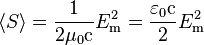
where Em is the amplitude of the electric field and c is the speed of light in free space. This time-averaged value is called irradiance and denoted Ee in radiometry, or is called intensity and denoted I in other fields.
Derivation
In an electromagnetic plane wave, E and B are always perpendicular to each other and the direction of propagation. Moreover, their amplitudes are related according to

and their time and position dependences are


where ω is the angular frequency of the wave and k is wave vector.
The time-dependent and position magnitude of the Poynting vector is then

In the last step, we used the equality ε0μ0 = 1/c2. Since the time- or space-average of cos2(ωt − k ⋅ r) is 1/2, it follows that
It will be appreciated that quantitatively the Poynting vector is evaluated only from a prior knowledge of the distribution of electric and magnetic fields, which are calculated by applying boundary conditions to a particular set of physical circumstances, for example a dipole antenna. Therefore the E and H field distributions form the primary object of any analysis, while the Poynting vector remains an interesting by-product.
Radiation pressure
The density of the linear momentum of the electromagnetic field is S/c2 where S is the magnitude of the Poynting vector and c is the speed of light in free space. The radiation pressure exerted by an electromagnetic wave on the surface of a target is given by:

Static fields

The consideration of the Poynting vector in static fields shows the relativistic nature of the Maxwell equations and allows a better understanding of the magnetic component of the Lorentz force, q(v × B). To illustrate, the accompanying picture is considered, which describes the Poynting vector in a cylindrical capacitor, which is located in an H field (pointing into the page) generated by a permanent magnet. Although there are only static electric and magnetic fields, the calculation of the Poynting vector produces a clockwise circular flow of electromagnetic energy, with no beginning or end.
While the circulating energy flow may seem nonsensical or paradoxical, it proves to be absolutely necessary to maintain conservation of momentum. Momentum density is proportional to energy flow density, so the circulating flow of energy contains an angular momentum.[14] This is the cause of the magnetic component of the Lorentz force which occurs when the capacitor is discharged. During discharge, the angular momentum contained in the energy flow is depleted as it is transferred to the charges of the discharge current crossing the magnetic field.
Notes
- ↑ Julius Adams Stratton (1941). "Chap.II Stress and Energy". Electromagnetic Theory (First ed.). New York: McGraw-Hill. p. 132.
”first derived by Poynting in 1884 and again in the same year by Heaviside.”
- ↑ Electromagnetism (2nd Edition), I.S. Grant, W.R. Phillips, Manchester Physics, John Wiley & Sons, 2008, ISBN 978-0471927129
- ↑ Introduction to Electrodynamics (3rd Edition), D.J. Griffiths, Pearson Education, Dorling Kindersley, 2007, ISBN 81-7758-293-3
- ↑ Poynting, J. H. (1884). "On the Transfer of Energy in the Electromagnetic Field". Philosophical Transactions of the Royal Society of London 175: 343–361. doi:10.1098/rstl.1884.0016.
- ↑ 5.0 5.1 5.2 5.3 5.4 John David Jackson (1998). Classical electrodynamics (Third ed.). New York: Wiley. ISBN 0-471-30932-X.
- ↑ Kinsler, P.; Favaro, A.; McCall M.W. (2009). "Four Poynting theorems". Eur. J. Phys. 30 (5): 983. arXiv:0908.1721. Bibcode:2009EJPh...30..983K. doi:10.1088/0143-0807/30/5/007.
- ↑ Pfeifer, R.N.C.; Nieminen, T.A.; Heckenberg N. R.; Rubinsztein-Dunlop H. (2007). "Momentum of an electromagnetic wave in dielectric media". Rev. Mod. Phys. 79 (4): 1197. Bibcode:2007RvMP...79.1197P. doi:10.1103/RevModPhys.79.1197.
- ↑ Umov, N. A. (1874). "Ein Theorem über die Wechselwirkungen in Endlichen Entfernungen". Zeitschrift für Mathematik und Physik XIX: 97.
- ↑ Bondar, H.; Bastien, F. (2008). "Quelques remarques sur la transmission de l’énergie électromagnétique en champ proche". Annales de la Fondation Louis de Broglie. 33 (3-4): 283–305.
- ↑ 10.0 10.1 Richter, F.; Florian, M.; Henneberger, K. (2008). "Poynting's theorem and energy conservation in the propagation of light in bounded media". Europhys. Lett. 81 (6): 67005. arXiv:0710.0515. Bibcode:2008EL.....8167005R. doi:10.1209/0295-5075/81/67005.
- ↑ Harrington (1981, p. 61)
- ↑ Hayt (1993, p. 402)
- ↑ Reitz (1993, p. 454)
- ↑ Feynman Lectures on Physics, Sections 17-4 and Volume 2, Chapter 17, section 4 and the end of Chapter 27, Section 6.
References
- Harrington, Roger F. (1961). "Time-Harmonic Electromagnetic Fields". McGraw-Hill
- Hayt, William (1981). Engineering Electromagnetics (4th ed.). McGraw-Hill. ISBN 0-07-027395-2
- Reitz, John R.; Milford, Frederick J.; Christy, Robert W. (1993). Foundations of Electromagnetic Theory (4th ed.). Addison-Wesley. ISBN 0-201-52624-7
Further reading
- "Poynting Vector" from ScienceWorld (A Wolfram Web Resource) by Eric W. Weisstein
- Richard Becker & Sauter, F (1964). Electromagnetic fields and interactions. New York: Dover. ISBN 0-486-64290-9.
- Joseph Edminister (1995). Schaum's outline of theory and problems of electromagnetics. New York: McGraw-Hill Professional. p. 225. ISBN 0-07-021234-1.