Poisson's ratio
Poisson's ratio, named after Siméon Poisson, is the negative ratio of transverse to axial strain. When a material is compressed in one direction, it usually tends to expand in the other two directions perpendicular to the direction of compression. This phenomenon is called the Poisson effect. Poisson's ratio  (nu) is a measure of this effect. The Poisson ratio is the fraction (or percent) of expansion divided by the fraction (or percent) of compression, for small values of these changes.
Conversely, if the material is stretched rather than compressed, it usually tends to contract in the directions transverse to the direction of stretching. This is a common observation when a rubber band is stretched, when it becomes noticeably thinner. Again, the Poisson ratio will be the ratio of relative contraction to relative expansion, and will have the same value as above. In certain rare cases, a material will actually shrink in the transverse direction when compressed (or expand when stretched) which will yield a negative value of the Poisson ratio.
The Poisson's ratio of a stable, isotropic, linear elastic material cannot be less than −1.0 nor greater than 0.5 due to the requirement that Young's modulus, the shear modulus and bulk modulus have positive values.[1] Most materials have Poisson's ratio values ranging between 0.0 and 0.5. A perfectly incompressible material deformed elastically at small strains would have a Poisson's ratio of exactly 0.5. Most steels and rigid polymers when used within their design limits (before yield) exhibit values of about 0.3, increasing to 0.5 for post-yield deformation (Seismic Performance of Steel-Encased Concrete Piles by RJT Park) (which occurs largely at constant volume.) Rubber has a Poisson ratio of nearly 0.5. Cork's Poisson ratio is close to 0: showing very little lateral expansion when compressed. Some materials, mostly polymer foams, have a negative Poisson's ratio; if these auxetic materials are stretched in one direction, they become thicker in perpendicular direction. Some anisotropic materials have one or more Poisson ratios above 0.5 in some directions.
Assuming that the material is stretched or compressed along the axial direction (the x axis in the below diagram):
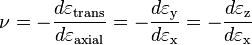
where
- is the resulting Poisson's ratio,
 is transverse strain (negative for axial tension (stretching), positive for axial compression)
 is axial strain (positive for axial tension, negative for axial compression).
Length change

 due to tension, and contracted in the y and z directions by
  .
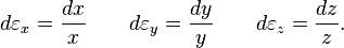
.For a cube stretched in the x-direction (see figure 1) with a length increase of in the x direction, and a length decrease of in the y and z directions, the infinitesimal diagonal strains are given by
Integrating these expressions and using the definition of Poisson's ratio gives
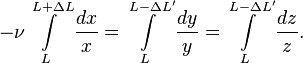
Solving and exponentiating, the relationship between and is then
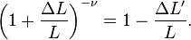
For very small values of and , the first-order approximation yields:

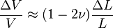
Volumetric change
The relative change of volume ΔV/V of a cube due to the stretch of the material can now be calculated. Using  and
and  :
:
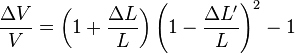
Using the above derived relationship between and :
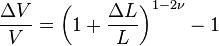
and for very small values of and , the first-order approximation yields:
For isotropic materials we can use Lamé’s relation[2]
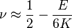
where  is bulk modulus.
Note that isotropic materials must have a Poisson's ratio of  . Typical isotropic engineering materials have a Poisson's ratio of
  .[3]
.[3]
Width change

If a rod with diameter (or width, or thickness) d and length L is subject to tension so that its length will change by ΔL then its diameter d will change by:
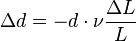
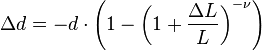
The above formula is true only in the case of small deformations; if deformations are large then the following (more precise) formula can be used:
where
 is original diameter
 is rod diameter change
- is Poisson's ratio
 is original length, before stretch
- is the change of length.
The value is negative because it decreases with increase of length
Isotropic materials
For a linear isotropic material subjected only to compressive (i.e. normal) forces, the deformation of a material in the direction of one axis will produce a deformation of the material along the other axis in three dimensions. Thus it is possible to generalize Hooke's Law (for compressive forces) into three dimensions:
![\varepsilon_x = \frac {1}{E} \left [ \sigma_x - \nu \left ( \sigma_y + \sigma_z \right ) \right ]](../I/m/f96cf49b267ede9e47bbfb3b7249873f.png)
![\varepsilon_y = \frac {1}{E} \left [ \sigma_y - \nu \left ( \sigma_x + \sigma_z \right ) \right ]](../I/m/1677af686fe5f6b3ee69c910b84445ee.png)
![\varepsilon_z = \frac {1}{E} \left [ \sigma_z - \nu \left ( \sigma_x + \sigma_y \right ) \right ]](../I/m/2fc0dc49396a59c7df5f108a78d82d96.png)
or
![\varepsilon_i = \frac {1}{E} \left [ \sigma_i(1+\nu) - \nu \left ( \sigma_x + \sigma_y+\sigma_z \right ) \right ]](../I/m/cc4142e21b2f2d4e80b5fa36c0c1b21c.png)
where
 ,
,  and
and  are strain in the direction of
  ,
,  and
and  axis
axis ,
,  and
and  are stress in the direction of , and axis
 is Young's modulus (the same in all directions: , and for isotropic materials)
- is Poisson's ratio (the same in all directions: , and for isotropic materials)
These equations will hold in the general case which includes shear forces as well as compressive forces, and the full generalization of Hooke's law is given by:
![\varepsilon_{ij} = \frac {1}{E} \left [ \sigma_{ij}(1+\nu) - \nu \delta_{ij}\sigma_{kk} \right ]](../I/m/aced89f2a750bf36f20e3feeeb08170c.png)
where  is the Kronecker delta and

Orthotropic materials
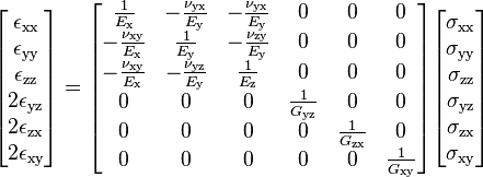
For orthotropic materials such as wood, Hooke's law can be expressed in matrix form as[4][5]
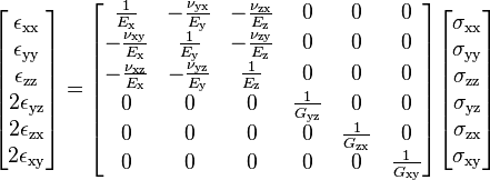
where
 is the Young's modulus along axis
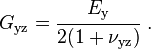
 is the shear modulus in direction
  on the plane whose normal is in direction
  is the Poisson's ratio that corresponds to a contraction in direction when an extension is applied in direction .
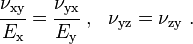
The Poisson's ratio of an orthotropic material is different in each direction (x, y and z). However, the symmetry of the stress and strain tensors implies that not all the six Poisson's ratios in the equation are independent. There are only nine independent material properties; three elastic moduli, three shear moduli, and three Poisson's ratios. The remaining three Poisson's ratios can be obtained from the relations
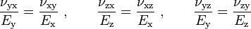
From the above relations we can see that if  then
then  . The larger Poisson's ratio (in this case
  ) is called the major Poisson's ratio while the smaller one (in this case
  ) is called the minor Poisson's ratio. We can find similar relations between the other Poisson's ratios.
Transversely isotropic materials
Transversely isotropic materials have a plane of isotropy in which the elastic properties are isotropic. If we assume that this plane of isotropy is  , then Hooke's law takes the form[6]
where we have used the plane of isotropy to reduce the number of constants, i.e.,  .
.
The symmetry of the stress and strain tensors implies that
This leaves us with six independent constants  . However, transverse isotropy gives rise to a further constraint between
  and
and  which is
Therefore, there are five independent elastic material properties two of which are Poisson's ratios. For the assumed plane of symmetry, the larger of and is the major Poisson's ratio. The other major and minor Poisson's ratios are equal.
Poisson's ratio values for different materials

| Material | Poisson's ratio |
|---|---|
| rubber | 0.4999 [3] |
| gold | 0.42–0.44 |
| saturated clay | 0.40–0.49 |
| magnesium | 0.35 |
| titanium | 0.34 |
| copper | 0.33 |
| aluminium-alloy | 0.32 |
| clay | 0.30–0.45 |
| stainless steel | 0.30–0.31 |
| steel | 0.27–0.30 |
| cast iron | 0.21–0.26 |
| sand | 0.20–0.45 |
| concrete | 0.20 |
| glass | 0.18–0.3 |
| foam | 0.10–0.50 |
| cork | ~ 0.00 |
| Material | Plane of symmetry | | |  |  |  |  |
|---|---|---|---|---|---|---|---|
| Nomex honeycomb core |  , = ribbon direction , = ribbon direction |
0.49 | 0.69 | 0.01 | 2.75 | 3.88 | 0.01 |
| glass fiber-epoxy resin | |
0.29 | 0.32 | 0.06 | 0.06 | 0.32 |
Negative Poisson's ratio materials
Some materials known as auxetic materials display a negative Poisson’s ratio. When subjected to positive strain in a longitudinal axis, the transverse strain in the material will actually be positive (i.e. it would increase the cross sectional area). For these materials, it is usually due to uniquely oriented, hinged molecular bonds. In order for these bonds to stretch in the longitudinal direction, the hinges must ‘open’ in the transverse direction, effectively exhibiting a positive strain.[8] This can also be done in a structured way and lead to new aspects in material design as for mechanical metamaterials.
Applications of Poisson's effect
One area in which Poisson's effect has a considerable influence is in pressurized pipe flow. When the air or liquid inside a pipe is highly pressurized it exerts a uniform force on the inside of the pipe, resulting in a radial stress within the pipe material. Due to Poisson's effect, this radial stress will cause the pipe to slightly increase in diameter and decrease in length. The decrease in length, in particular, can have a noticeable effect upon the pipe joints, as the effect will accumulate for each section of pipe joined in series. A restrained joint may be pulled apart or otherwise prone to failure.
Another area of application for Poisson's effect is in the realm of structural geology. Rocks, like most materials, are subject to Poisson's effect while under stress. In a geological timescale, excessive erosion or sedimentation of Earth's crust can either create or remove large vertical stresses upon the underlying rock. This rock will expand or contract in the vertical direction as a direct result of the applied stress, and it will also deform in the horizontal direction as a result of Poisson's effect. This change in strain in the horizontal direction can affect or form joints and dormant stresses in the rock.[9]
The use of cork as a stopper for wine bottles is due to cork having a Poisson ratio of practically zero, so that, as the cork is inserted into the bottle, the upper part which is not yet inserted does not expand as the lower part is compressed. The force needed to insert a cork into a bottle arises only from the compression of the cork and the friction between the cork and the bottle. If the stopper were made of rubber, for example, (with a Poisson ratio of about 1/2), there would be a relatively large additional force required to overcome the expansion of the upper part of the rubber stopper.
See also
- 3-D elasticity
- Hooke's Law
- Impulse excitation technique
- Orthotropic material
- Shear modulus
- Young's modulus
- Coefficient of thermal expansion
References
- ↑ H. GERCEK; “Poisson's ratio values for rocks”; International Journal of Rock Mechanics and Mining Sciences; Elsevier; January 2007; 44 (1): pp. 1–13
- ↑ http://arxiv.org/ftp/arxiv/papers/1204/1204.3859.pdf - Limits to Poisson’s ratio in isotropic materials – general result for arbitrary deformation.
- ↑ 3.0 3.1 http://polymerphysics.net/pdf/PhysRevB_80_132104_09.pdf
- ↑ Boresi, A. P, Schmidt, R. J. and Sidebottom, O. M., 1993, Advanced Mechanics of Materials, Wiley.
- ↑ Lekhnitskii, SG., (1963), Theory of elasticity of an anisotropic elastic body, Holden-Day Inc.
- ↑ Tan, S. C., 1994, Stress Concentrations in Laminated Composites, Technomic Publishing Company, Lancaster, PA.
- ↑ Poisson's ratio calculation of glasses
- ↑ Negative Poisson's ratio
- ↑ http://www.geosc.psu.edu/~engelder/geosc465/lect18.rtf
External links
- Meaning of Poisson's ratio
- Negative Poisson's ratio materials
- More on negative Poisson's ratio materials (auxetic)
| ||||||
| Conversion formulas | |||||||
|---|---|---|---|---|---|---|---|
| Homogeneous isotropic linear elastic materials have their elastic properties uniquely determined by any two moduli among these; thus, given any two, any other of the elastic moduli can be calculated according to these formulas. | |||||||
 |
 |
 |
 |
 |
 |
Notes | |
 |
|
|
 |
 |
 |
 |
|
 |
|
 |
 |
 |
 |
 |
|
 |
|
 |
 |
 |
 |
 |
|
 |
|
 |
 |
 |
|
 |
|
 |
|
 |
 |
 |
 |
 |
|
 |
 |
|
|
 |
 |
 |
 |
 |
 |
|
 |
|
 |
 |
|
 |
 |
|
 |
 |
|
 |
|
 |
 |
|
 |
 |
 |
|
|
 |
 |
 |
|
|
 |
 |
|
 |
 |
 |
|
 |
|
 |
Cannot be used when  |
 |
 |
 |
|
 |
 |
|
|
 |
 |
 |
 |
|
|
 |
|
 |
 |
 |
 |
|
 |
|
|
 |
 |
 |
 |
 |
|
|
|

 .
. .
.