Poisson's equation

In mathematics, Poisson's equation is a partial differential equation of elliptic type with broad utility in electrostatics, mechanical engineering and theoretical physics. It is used, for instance, to describe the potential energy field caused by a given charge or mass density distribution. The equation is named after the French mathematician, geometer, and physicist Siméon Denis Poisson.^[1]

Statement of the equation

Poisson's equation is

\Delta\varphi=f

where $\Delta$ is the Laplace operator, and f and φ are real or complex-valued functions on a manifold. Usually, f is given and φ is sought. When the manifold is Euclidean space, the Laplace operator is often denoted as ∇² and so Poisson's equation is frequently written as

\nabla^2 \varphi = f.

In three-dimensional Cartesian coordinates, it takes the form

\left( \frac{\partial^2}{\partial x^2} + \frac{\partial^2}{\partial y^2} + \frac{\partial^2}{\partial z^2} \right)\varphi(x,y,z) = f(x,y,z).

When $f =0$ we retrieve Laplace's equation.

Poisson's equation may be solved using a Green's function; a general exposition of the Green's function for Poisson's equation is given in the article on the screened Poisson equation. There are various methods for numerical solution. The relaxation method, an iterative algorithm, is one example.

Newtonian gravity

Main articles: gravitational field and Gauss's law for gravity

In the case of a gravitational field g due to an attracting massive object of density ρ, Gauss's law for gravity in differential form can be used to obtain the corresponding Poisson equation for gravity:

\nabla\cdot\bold{g} = -4\pi G\rho

Since the gravitational field is conservative, it can be expressed in terms of a scalar potential Φ:

\bold{g} = -\nabla \Phi

Substituting into Gauss's law

\nabla\cdot(-\nabla \Phi) = - 4\pi G \rho

obtains Poisson's equation for gravity:

{\nabla}^2 \Phi = 4\pi G \rho.

Electrostatics

Main article: Electrostatics

One of the cornerstones of electrostatics is setting up and solving problems described by the Poisson equation. Solving the Poisson equation amounts to finding the electric potential φ for a given charge distribution $\rho_f$ .

The mathematical details behind Poisson's equation in electrostatics are as follows (SI units are used rather than Gaussian units, which are also frequently used in electromagnetism).

Starting with Gauss's law for electricity (also one of Maxwell's equations) in differential form, we have:

\mathbf{\nabla} \cdot \mathbf{D} = \rho_f

where $\mathbf{\nabla} \cdot$ is the divergence operator, D = electric displacement field, and ρ_f = free charge density (describing charges brought from outside). Assuming the medium is linear, isotropic, and homogeneous (see polarization density), we have the constitutive equation:

\mathbf{D} = \varepsilon \mathbf{E}

where ε = permittivity of the medium and E = electric field. Substituting this into Gauss's law and assuming ε is spatially constant in the region of interest obtains:

\mathbf{\nabla} \cdot \mathbf{E} = \frac{\rho_f}{\varepsilon}

In the absence of a changing magnetic field, B, Faraday's law of induction gives:

\nabla \times \mathbf{E} = -\dfrac{\partial \mathbf{B}} {\partial t} = 0

where $\nabla \times$ is the curl operator and t is time. Since the curl of the electric field is zero, it is defined by a scalar electric potential field, $\varphi$ (see Helmholtz decomposition).

\mathbf{E} = -\nabla \varphi

The derivation of Poisson's equation under these circumstances is straightforward. Substituting the potential gradient for the electric field

\nabla \cdot \bold{E} = \nabla \cdot ( - \nabla \varphi ) = - {\nabla}^2 \varphi = \frac{\rho_f}{\varepsilon},

directly obtains Poisson's equation for electrostatics, which is:

{\nabla}^2 \varphi = -\frac{\rho_f}{\varepsilon}.

Solving Poisson's equation for the potential requires knowing the charge density distribution. If the charge density is zero, then Laplace's equation results. If the charge density follows a Boltzmann distribution, then the Poisson-Boltzmann equation results. The Poisson–Boltzmann equation plays a role in the development of the Debye–Hückel theory of dilute electrolyte solutions.

The above discussion assumes that the magnetic field is not varying in time. The same Poisson equation arises even if it does vary in time, as long as the Coulomb gauge is used. In this more general context, computing φ is no longer sufficient to calculate E, since E also depends on the magnetic vector potential A, which must be independently computed. See Maxwell's equation in potential formulation for more on φ and A in Maxwell's equations and how Poisson's equation is obtained in this case.

Potential of a Gaussian charge density

If there is a static spherically symmetric Gaussian charge density

\rho_f(r) = \frac{Q}{\sigma^3\sqrt{2\pi}^3}\,e^{-r^2/(2\sigma^2)},

where Q is the total charge, then the solution φ(r) of Poisson's equation,

{\nabla}^2 \varphi = - { \rho_f \over \varepsilon }

is given by

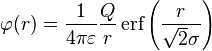
\varphi(r) = { 1 \over 4 \pi \varepsilon } \frac{Q}{r}\,\mbox{erf}\left(\frac{r}{\sqrt{2}\sigma}\right)

where erf(x) is the error function.

This solution can be checked explicitly by evaluating ${\nabla}^2 \varphi$ . Note that, for r much greater than σ, the erf function approaches unity and the potential φ (r) approaches the point charge potential

\varphi \approx { 1 \over 4 \pi \varepsilon } {Q \over r}

as one would expect. Furthermore the erf function approaches 1 extremely quickly as its argument increases; in practice for r > 3σ the relative error is smaller than one part in a thousand.

Surface reconstruction

Poisson's equation is also used to reconstruct a smooth 2D surface (in the sense of curve fitting) based on a large number of points p_i (a point cloud) where each point also carries an estimate of the local surface normal n_i.^[2]

This technique reconstructs the implicit function f whose value is zero at the points p_i and whose gradient at the points p_i equals the normal vectors n_i. The set of (p_i, n_i) is thus a sampling of a continuous vector ﬁeld V. The implicit function f is found by integrating the vector ﬁeld V. Since not every vector ﬁeld is the gradient of a function, the problem may or may not have a solution: the necessary and sufﬁcient condition for a smooth vector ﬁeld V to be the gradient of a function f is that the curl of V must be identically zero. In case this condition is difﬁcult to impose, it is still possible to perform a least-squares fit to minimize the difference between V and the gradient of f.

References

↑ Jackson, Julia A.; Mehl, James P.; Neuendorf, Klaus K. E., eds. (2005), Glossary of Geology, American Geological Institute, Springer, p. 503, ISBN 9780922152766 .
↑ F. Calakli and G. Taubin, Smooth Signed Distance Surface Reconstruction, Paciﬁc Graphics Vol 30-7, 2011

Poisson Equation at EqWorld: The World of Mathematical Equations.
L.C. Evans, Partial Differential Equations, American Mathematical Society, Providence, 1998. ISBN 0-8218-0772-2
A. D. Polyanin, Handbook of Linear Partial Differential Equations for Engineers and Scientists, Chapman & Hall/CRC Press, Boca Raton, 2002. ISBN 1-58488-299-9

External links

Hazewinkel, Michiel, ed. (2001), "Poisson equation", Encyclopedia of Mathematics, Springer, ISBN 978-1-55608-010-4
Poisson's equation on PlanetMath.