Periodogram
The periodogram is an estimate of the spectral density of a signal. The term was coined by Arthur Schuster in 1898[1] as in the following quote:[2]
| “ | THE PERIODOGRAM. It is convenient to have a word for some representation of a variable quantity which shall correspond to the 'spectrum' of a luminous radiation. I propose the word periodogram, and define it more particularly in the following way:
Let where T may for convenience be chosen to be equal to some integer multiple of
and plot a curve with as ordinates; this curve, or, better, the space between this curve and the axis of abscissæ, represents the periodogram of f(t). |
” |
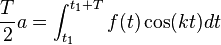
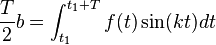
 ,
, as abscissae and
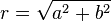
Note that the term periodogram may also be used to describe the quantity  ,[3] which is its common meaning in astronomy (as in "the modulus-squared of the discrete Fourier transform of the time series (with the appropriate normalisation)"[4]). See Scargle (1982) for a detailed discussion in this context.[5]
A spectral plot refers to a smoothed version of the periodogram.[6][7] Smoothing is performed to reduce the effect of measurement noise.
In practice, the periodogram is often computed from a finite-length digital sequence using the fast Fourier transform (FFT). The raw periodogram is not a good spectral estimate because of spectral bias and the fact that the variance at a given frequency does not decrease as the number of samples used in the computation increases.
The spectral bias problem arises from a sharp truncation of the sequence, and can be reduced by first multiplying the finite sequence by a window function which truncates the sequence gradually rather than abruptly.
The variance problem can be reduced by smoothing the periodogram. Various techniques to reduce spectral bias and variance are the subject of spectral estimation.
One such technique to solve the variance problems is also known as the method of averaged periodograms[8] or as Bartlett's method. The idea behind it is, to divide the set of N samples into L sets of M samples, compute the discrete Fourier transform (DFT) of each set, square it to get the power spectral density and compute the average of all of them. This leads to a decrease in the standard deviation as 
See also
References
- ↑ Schuster, A., "On the investigation of hidden periodicities with application to a supposed 26 day period of meteorological phenomena," Terrestrial Magnetism, 3, 13-41, 1898.
- ↑ The Annals of Mathematical Statistics. 1972.
- ↑ Box, George and Jenkins, Gwilym (1970) Time series analysis: Forecasting and control, San Francisco: Holden-Day.
- ↑ Simon Vaughan and Philip Uttley (2006), "Detecting X-ray QPOs in active galaxies",Advances in Space Research, Volume 38, Issue 7, pp. 1405-1408
- ↑ Scargle (1982), Astrophysical Journal, Part 1, vol. 263, Dec. 15, 1982, p. 835-853
- ↑ Spectral Plot, from the NIST Engineering Statistics Handbook.
- ↑ Short explanation of the relation between the spectral plot and the periodogram.
- ↑ Engelberg, S. (2008), Digital Signal Processing: An Experimental Approach, Springer, Chap. 7 p. 56