Parabolic coordinates

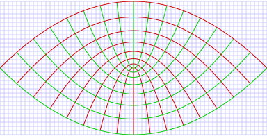
Parabolic coordinates are a two-dimensional orthogonal coordinate system in which the coordinate lines are confocal parabolas. A three-dimensional version of parabolic coordinates is obtained by rotating the two-dimensional system about the symmetry axis of the parabolas.

Parabolic coordinates have found many applications, e.g., the treatment of the Stark effect and the potential theory of the edges.

Two-dimensional parabolic coordinates

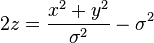
Two-dimensional parabolic coordinates $(\sigma, \tau)$ are defined by the equations

x = \sigma \tau\,

y = \frac{1}{2} \left( \tau^{2} - \sigma^{2} \right)

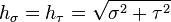
The curves of constant $\sigma$ form confocal parabolae

2y = \frac{x^{2}}{\sigma^{2}} - \sigma^{2}

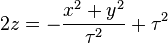
that open upwards (i.e., towards $+y$ ), whereas the curves of constant $\tau$ form confocal parabolae

2y = -\frac{x^{2}}{\tau^{2}} + \tau^{2}

that open downwards (i.e., towards $-y$ ). The foci of all these parabolae are located at the origin.

Two-dimensional scale factors

The scale factors for the parabolic coordinates $(\sigma, \tau)$ are equal

h_{\sigma} = h_{\tau} = \sqrt{\sigma^{2} + \tau^{2}}

Hence, the infinitesimal element of area is

dA = \left( \sigma^{2} + \tau^{2} \right) d\sigma d\tau

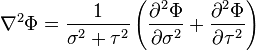
and the Laplacian equals

\nabla^{2} \Phi = \frac{1}{\sigma^{2} + \tau^{2}} \left( \frac{\partial^{2} \Phi}{\partial \sigma^{2}} + \frac{\partial^{2} \Phi}{\partial \tau^{2}} \right)

Other differential operators such as $\nabla \cdot \mathbf{F}$ and $\nabla \times \mathbf{F}$ can be expressed in the coordinates $(\sigma, \tau)$ by substituting the scale factors into the general formulae found in orthogonal coordinates.

Three-dimensional parabolic coordinates

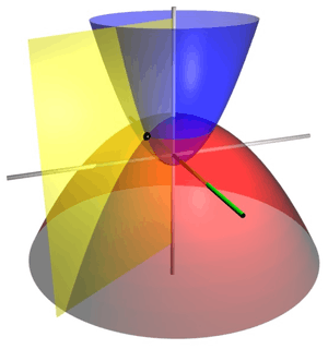
Coordinate surfaces of the three-dimensional parabolic coordinates. The red paraboloid corresponds to τ=2, the blue paraboloid corresponds to σ=1, and the yellow half-plane corresponds to φ=-60°. The three surfaces intersect at the point P (shown as a black sphere) with Cartesian coordinates roughly (1.0, -1.732, 1.5).

The two-dimensional parabolic coordinates form the basis for two sets of three-dimensional orthogonal coordinates. The parabolic cylindrical coordinates are produced by projecting in the $z$ -direction. Rotation about the symmetry axis of the parabolae produces a set of confocal paraboloids, forming a coordinate system that is also known as "parabolic coordinates"

x = \sigma \tau \cos \varphi

y = \sigma \tau \sin \varphi

z = \frac{1}{2} \left(\tau^{2} - \sigma^{2} \right)

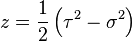
where the parabolae are now aligned with the $z$ -axis, about which the rotation was carried out. Hence, the azimuthal angle $\phi$ is defined

\tan \varphi = \frac{y}{x}

The surfaces of constant $\sigma$ form confocal paraboloids

2z = \frac{x^{2} + y^{2}}{\sigma^{2}} - \sigma^{2}

that open upwards (i.e., towards $+z$ ) whereas the surfaces of constant $\tau$ form confocal paraboloids

2z = -\frac{x^{2} + y^{2}}{\tau^{2}} + \tau^{2}

that open downwards (i.e., towards $-z$ ). The foci of all these paraboloids are located at the origin.

The Riemannian metric tensor associated with this coordinate system is

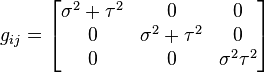
g_{ij} = \begin{bmatrix} \sigma^2+\tau^2 & 0 & 0\\0 & \sigma^2+\tau^2 & 0\\0 & 0 & \sigma^2\tau^2 \end{bmatrix}

Three-dimensional scale factors

The three dimensional scale factors are:

h_{\sigma} = \sqrt{\sigma^2+\tau^2}

h_{\tau} = \sqrt{\sigma^2+\tau^2}

h_{\varphi} = \sigma\tau\,

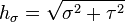
It is seen that The scale factors $h_{\sigma}$ and $h_{\tau}$ are the same as in the two-dimensional case. The infinitesimal volume element is then

dV = h_\sigma h_\tau h_\varphi\, d\sigma\,d\tau\,d\varphi = \sigma\tau \left( \sigma^{2} + \tau^{2} \right)\,d\sigma\,d\tau\,d\varphi

and the Laplacian is given by

\nabla^2 \Phi = \frac{1}{\sigma^{2} + \tau^{2}} \left[ \frac{1}{\sigma} \frac{\partial}{\partial \sigma} \left( \sigma \frac{\partial \Phi}{\partial \sigma} \right) + \frac{1}{\tau} \frac{\partial}{\partial \tau} \left( \tau \frac{\partial \Phi}{\partial \tau} \right)\right] + \frac{1}{\sigma^2\tau^2}\frac{\partial^2 \Phi}{\partial \varphi^2}

Other differential operators such as $\nabla \cdot \mathbf{F}$ and $\nabla \times \mathbf{F}$ can be expressed in the coordinates $(\sigma, \tau, \phi)$ by substituting the scale factors into the general formulae found in orthogonal coordinates.

Bibliography

Morse PM, Feshbach H (1953). Methods of Theoretical Physics, Part I. New York: McGraw-Hill. p. 660. ISBN 0-07-043316-X. LCCN 52011515.
Margenau H, Murphy GM (1956). The Mathematics of Physics and Chemistry. New York: D. van Nostrand. pp. 185–186. LCCN 55010911.
Korn GA, Korn TM (1961). Mathematical Handbook for Scientists and Engineers. New York: McGraw-Hill. p. 180. LCCN 59014456. ASIN B0000CKZX7.
Sauer R, Szabó I (1967). Mathematische Hilfsmittel des Ingenieurs. New York: Springer Verlag. p. 96. LCCN 67025285.
Zwillinger D (1992). Handbook of Integration. Boston, MA: Jones and Bartlett. p. 114. ISBN 0-86720-293-9. Same as Morse & Feshbach (1953), substituting u_k for ξ_k.
Moon P, Spencer DE (1988). "Parabolic Coordinates (μ, ν, ψ)". Field Theory Handbook, Including Coordinate Systems, Differential Equations, and Their Solutions (corrected 2nd ed., 3rd print ed.). New York: Springer-Verlag. pp. 34–36 (Table 1.08). ISBN 978-0-387-18430-2.

External links

Hazewinkel, Michiel, ed. (2001), "Parabolic coordinates", Encyclopedia of Mathematics, Springer, ISBN 978-1-55608-010-4
MathWorld description of parabolic coordinates

Orthogonal coordinate systems

Two dimensional	Cartesian coordinate system Polar coordinate system Parabolic coordinate system Bipolar coordinates Elliptic coordinates

Three dimensional	Cartesian coordinate system Cylindrical coordinate system Spherical coordinate system Parabolic cylindrical coordinates Paraboloidal coordinates Oblate spheroidal coordinates Prolate spheroidal coordinates Ellipsoidal coordinates Elliptic cylindrical coordinates Toroidal coordinates Bispherical coordinates Bipolar cylindrical coordinates Conical coordinates 6-sphere coordinates Flat-ring cyclide coordinates Flat-disk cyclide coordinates Bi-cyclide coordinates Cap-cyclide coordinates Concave bi-sinusoidal single-centered coordinates Concave bi-sinusoidal double-centered coordinates Convex inverted-sinusoidal spherically aligned coordinates Quasi-random-intersection cartesian coordinates