Panel data
In statistics and econometrics, the term panel data refers to multi-dimensional data frequently involving measurements over time. Panel data contain observations of multiple phenomena obtained over multiple time periods for the same firms or individuals. In biostatistics, the term longitudinal data is often used instead,[1][2] wherein a subject or cluster constitutes a panel member or individual in a longitudinal study.
Time series and cross-sectional data are special cases of panel data that are in one dimension only (one panel member or individual for the former, one time point for the latter).
Example
| balanced panel: | unbalanced panel: | |
|---|---|---|
 |
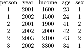 |
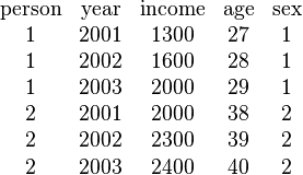
In the example above, two data sets with a two-dimensional panel structure are shown, although the second data set might be a three-dimensional structure since it has three people. Individual characteristics (income, age, sex. educ) are collected for different persons and different years. In the left data set two persons (1, 2) are observed over three years (2001, 2002, 2003). Because each person is observed every year, the left-hand data set is called a balanced panel, whereas the data set on the right hand is called an unbalanced panel, since Person 1 is not observed in year 2003 and Person 3 is not observed in 2003 or 2001.
Analysis of panel data
A panel has the form

where  is the individual dimension and
  is the time dimension. A general panel data regression model is written as
  Different assumptions can be made on the precise structure of this general model. Two important models are the fixed effects model and the random effects model. The fixed effects model is denoted as
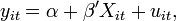
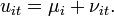
 are individual-specific, time-invariant effects (for example in a panel of countries this could include geography, climate etc.) and because we assume they are fixed over time, this is called the fixed-effects model. The random effects model assumes in addition that
and
that is, the two error components are independent from each other.
Data sets which have a panel design
- German Socio-Economic Panel (SOEP)
- Household, Income and Labour Dynamics in Australia Survey (HILDA)
- British Household Panel Survey (BHPS)
- Survey of Family Income and Employment (SoFIE)
- Survey of Income and Program Participation (SIPP)
- Lifelong Labour Market Database (LLMDB)
- Panel Study of Income Dynamics (PSID)
- Korean Labor and Income Panel Study (KLIPS)
- Chinese Family Panel Studies (CFPS)
- German Family Panel (pairfam)
- National Longitudinal Surveys (NLSY)
- Labour Force Survey (LFS)
- Korean Youth Panel (YP)
- Korean Longitudinal Study of Aging (KLoSA)
Data sets which have a multi-dimensional panel design
See also
Notes
- ↑ Diggle, Peter J.; Heagerty, Patrick; Liang, Kung-Yee; Zeger, Scott L. (2002). Analysis of Longitudinal Data (2nd ed.). Oxford University Press. p. 2. ISBN 0-19-852484-6.
- ↑ Fitzmaurice, Garrett M.; Laird, Nan M.; Ware, James H. (2004). Applied Longitudinal Analysis. Hoboken: John Wiley & Sons. p. 2. ISBN 0-471-21487-6.
References
- Baltagi, Badi H. (2008). Econometric Analysis of Panel Data (Fourth ed.). Chichester: John Wiley & Sons. ISBN 978-0-470-51886-1.
- Davies, A.; Lahiri, K. (1995). "A New Framework for Testing Rationality and Measuring Aggregate Shocks Using Panel Data". Journal of Econometrics 68 (1): 205–227. doi:10.1016/0304-4076(94)01649-K.
- Davies, A.; Lahiri, K. (2000). "Re-examining the Rational Expectations Hypothesis Using Panel Data on Multi-Period Forecasts". Analysis of Panels and Limited Dependent Variable Models. Cambridge: Cambridge University Press. pp. 226–254. ISBN 0-521-63169-6.
- Frees, E. (2004). Longitudinal and Panel Data: Analysis and Applications in the Social Sciences. New York: Cambridge University Press. ISBN 0-521-82828-7.
- Hsiao, Cheng (2003). Analysis of Panel Data (Second ed.). New York: Cambridge University Press. ISBN 0-521-52271-4.