Padé table
In complex analysis, a Padé table is an array, possibly of infinite extent, of the rational Padé approximants
- Rm, n
to a given complex formal power series. Certain sequences of approximants lying within a Padé table can often be shown to correspond with successive convergents of a continued fraction representation of a holomorphic or meromorphic function.
History
Although earlier mathematicians had obtained sporadic results involving sequences of rational approximations to transcendental functions, Frobenius (in 1881) was apparently the first to organize the approximants in the form of a table. Henri Padé further expanded this notion in his doctoral thesis Sur la representation approchee d'une fonction par des fractions rationelles, in 1892. Over the ensuing 16 years Padé published 28 additional papers exploring the properties of his table, and relating the table to analytic continued fractions.[1]
Modern interest in Padé tables was revived by H. S. Wall and Oskar Perron, who were primarily interested in the connections between the tables and certain classes of continued fractions. Daniel Shanks and Peter Wynn published influential papers about 1955, and W. B. Gragg obtained far-reaching convergence results during the '70s. More recently, the widespread use of electronic computers has stimulated a great deal of additional interest in the subject.[2]
Notation
A function f(z) is represented by a formal power series:
where c0 ≠ 0, by convention. The (m, n)th entry[3] Rm, n in the Padé table for f(z) is then given by
where Pm(z) and Qn(z) are polynomials of degrees not more than m and n, respectively. The coefficients {ai} and {bi} can always be found by considering the expression
and equating coefficients of like powers of z up through m + n. For the coefficients of powers m + 1 to m + n, the right hand side is 0 and the resulting system of linear equations contains a homogeneous system of n equations in the n + 1 unknowns bi, and so admits of infinitely many solutions each of which determines a possible Qn. Pm is then easily found by equating the first m coefficients of the equation above. However, it can be shown that, due to cancellation, the generated rational functions Rm, n are all the same, so that the (m, n)th entry in the Padé table is unique.[2] Alternatively, we may require that b0 = 1, thus putting the table in a standard form.
Although the entries in the Padé table can always be generated by solving this system of equations, that approach is computationally expensive. More efficient methods have been devised, including the epsilon algorithm.[4]
The block theorem and normal approximants
Because of the way the (m, n)th approximant is constructed, the difference
- Qn(z)f(z) − Pm(z)
is a power series whose first term is of degree no less than
- m + n + 1.
If the first term of that difference is of degree
- m + n + r + 1, r > 0,
then the rational function Rm, n occupies
- (r + 1)2
cells in the Padé table, from position (m, n) through position (m+r, n+r), inclusive. In other words, if the same rational function appears more than once in the table, that rational function occupies a square block of cells within the table. This result is known as the block theorem.
If a particular rational function occurs exactly once in the Padé table, it is called a normal approximant to f(z). If every entry in the complete Padé table is normal, the table itself is said to be normal. Normal Padé approximants can be characterized using determinants of the coefficients cn in the Taylor series expansion of f(z), as follows. Define the (m, n)th determinant by
with Dm,0 = 1, Dm,1 = cm, and ck = 0 for k < 0. Then
- the (m, n)th approximant to f(z) is normal if and only if none of the four determinants Dm,n−1, Dm,n, Dm+1,n, and Dm+1,n+1 vanish; and
- the Padé table is normal if and only if none of the determinants Dm,n are equal to zero (note in particular that this means none of the coefficients ck in the series representation of f(z) can be zero).[5]
Connection with continued fractions
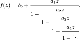
One of the most important forms in which an analytic continued fraction can appear is as a regular C-fraction, which is a continued fraction of the form
where the ai ≠ 0 are complex constants, and z is a complex variable.
There is an intimate connection between regular C-fractions and Padé tables with normal approximants along the main diagonal: the "stairstep" sequence of Padé approximants R0,0, R1,0, R1,1, R2,1, R2,2, … is normal if and only if that sequence coincides with the successive convergents of a regular C-fraction. In other words, if the Padé table is normal along the main diagonal, it can be used to construct a regular C-fraction, and if a regular C-fraction representation for the function f(z) exists, then the main diagonal of the Padé table representing f(z) is normal.[2]
An example – the exponential function
Here is an example of a Padé table, for the exponential function.
| m \ n | 0 | 1 | 2 | 3 |
|---|---|---|---|---|
| 0 |  |
 |
 |
 |
| 1 |  |
 |
 |
 |
| 2 |  |
 |
 |
 |
| 3 |  |
 |
 |
 |
| 4 |  |
 |
 |
 |
Several interesting features are immediately apparent.
- The first column of the table consists of the successive truncations of the Taylor series for ez.
- Similarly, the first row contains the reciprocals of successive truncations of the series expansion of e−z.
- The approximants Rm,n and Rn,m are quite symmetrical – the numerators and denominators are interchanged, and the patterns of plus and minus signs are different, but the same coefficients appear in both of these approximants. In fact, using the
 notation of generalized hypergeometric series,
- Computations involving the Rn,n (on the main diagonal) can be done quite efficiently. For example, R3,3 reproduces the power series for the exponential function perfectly up through 1/720 z6, but because of the symmetry of the two cubic polynomials, a very fast evaluation algorithm can be devised.
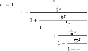
The procedure used to derive Gauss's continued fraction can be applied to a certain confluent hypergeometric series to derive the following C-fraction expansion for the exponential function, valid throughout the entire complex plane:
By applying the fundamental recurrence formulas one may easily verify that the successive convergents of this C-fraction are the stairstep sequence of Padé approximants R0,0, R1,0, R1,1, … Interestingly, in this particular case a closely related continued fraction can be obtained from the identity
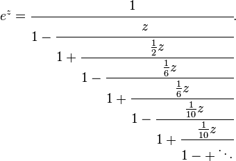
that continued fraction looks like this:
This fraction's successive convergents also appear in the Padé table, and form the sequence R0,0, R0,1, R1,1, R1,2, R2,2, …
Generalizations
A formal Newton series L is of the form
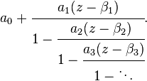
where the sequence {βk} of points in the complex plane is known as the set of interpolation points. A sequence of rational approximants Rm,n can be formed for such a series L in a manner entirely analogous to the procedure described above, and the approximants can be arranged in a Newton-Padé table. It has been shown[6] that some "staircase" sequences in the Newton-Padé table correspond with the successive convergents of a Thiele-type continued fraction, which is of the form
Mathematicians have also constructed two-point Padé tables by considering two series, one in powers of z, the other in powers of 1/z, which alternately represent the function f(z) in a neighborhood of zero and in a neighborhood of infinity.[2]
See also
Notes
- ↑ O'Connor, John J.; Robertson, Edmund F., "Padé table", MacTutor History of Mathematics archive, University of St Andrews.
- ↑ 2.0 2.1 2.2 2.3 Jones and Thron, 1980.
- ↑ The (m, n)th entry is considered to lie in row m and column n, and numbering of the rows and columns begins at (0, 0).
- ↑ Wynn, Peter (Apr 1956). "On a Device for Computing the em(Sn) Transformation". Mathematical Tables and Other Aids to Computation (American Mathematical Society) 10 (54): 91–96. doi:10.2307/2002183. JSTOR 2002183.
- ↑ Gragg, W.B. (Jan 1972). "The Padé Table and its Relation to Certain Algorithms of Numerical Analysis". SIAM Review 14 (1): 1–62. doi:10.1137/1014001. ISSN 0036-1445. JSTOR 2028911.
- ↑ Thiele, T.N. (1909). Interpolationsrechnung. Leipzig: Teubner. ISBN 1-4297-0249-4.
References
- Jones, William B.; Thron, W. J. (1980). Continued Fractions: Theory and Applications. Reading, Massachusetts: Addison-Wesley Publishing Company. pp. 185–197. ISBN 0-201-13510-8.
- Wall, H. S. (1973). Analytic Theory of Continued Fractions. Chelsea Publishing Company. pp. 377–415. ISBN 0-8284-0207-8.
(This is a reprint of the volume originally published by D. Van Nostrand Company, Inc., in 1948.)


