Orthotropic material

Wood is an example of an orthotropic material. Material properties in three perpendicular directions (axial, radial, and circumferential) are different.

An orthotropic material has three mutually orthogonal twofold axes of rotational symmetry so that its material properties are, in general, different along each axis. An object can be both orthotropic and inhomogeneous; it may have orthotropic properties that vary from point to point inside the volume of the object. This suggests that orthotropy is the property of a point within an object rather than for the object as a whole (unless the object is homogeneous). The associated planes of symmetry are also defined for a small region around a point and do not necessarily have to be identical to the planes of symmetry of the whole object.

A familiar example of an orthotropic material is wood. In wood, one can define three mutually perpendicular directions at each point in which the properties are different. These are the axial direction (along the grain), the radial direction, and the circumferential direction. Because the preferred coordinate system is cylindrical-polar, this type of orthotropy is also called polar orthotropy. In particular, the mechanical properties (such as strength and stiffness) along the grain are typically larger than in the radial and circumferential directions. Hankinson's equation provides a means to quantify the difference in strength in different directions.

Another example of an orthotropic material is a metal which has been rolled to form a sheet; the properties in the rolling direction and each of the two transverse directions will be different due to the anisotropic structure that develops during rolling.

Orthotropic materials are a subset of anisotropic materials; their properties depend on the direction in which they are measured. Orthotropic materials have three planes/axes of symmetry. An isotropic material, in contrast, has the same properties in every direction. It can be proved that a material having two planes of symmetry must have a third one. Isotropic materials have an infinite number of planes of symmetry.

Transversely isotropic materials are special orthotropic materials that have one axis of symmetry (any other pair of axes that are perpendicular to the main one and orthogonal among themselves are also axes of symmetry). One common example of transversely isotropic material with one axis of symmetry is a polymer reinforced by parallel glass or graphite fibers. The strength and stiffness of such a composite material will usually be greater in a direction parallel to the fibers than in the transverse direction, and the thickness direction usually has properties similar to the transverse direction. Another example would be a biological membrane, in which the properties in the plane of the membrane will be different from those in the perpendicular direction.

It is important to keep in mind that a material which is anisotropic on one length scale may be isotropic on another (usually larger) length scale. For instance, most metals are polycrystalline with very small grains. Each of the individual grains may be anisotropic, but if the material as a whole comprises many randomly oriented grains, then its measured mechanical properties will be an average of the properties over all possible orientations of the individual grains.

Orthotropy in physics

Anisotropic material relations

Material behavior is represented in physical theories by constitutive relations. A large class of physical behaviors can be represented by linear material models that take the form of a second-order tensor. The material tensor provides a relation between two vectors and can be written as

\mathbf{f} = \boldsymbol{K}\cdot\mathbf{d}

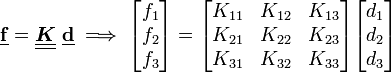
where $\mathbf{d},\mathbf{f}$ are two vectors representing physical quantities and $\boldsymbol{K}$ is the second-order material tensor. If we express the above equation in terms of components with respect to an orthonormal coordinate system, we can write

f_i = K_{ij}~d_j ~.

Summation over repeated indices has been assumed in the above relation. In matrix form we have

\underline{\mathbf{f}} = \underline{\underline{\boldsymbol{K}}}~\underline{\mathbf{d}} \implies \begin{bmatrix} f_1\\f_2\\f_3 \end{bmatrix} = \begin{bmatrix} K_{11} & K_{12} & K_{13} \\ K_{21} & K_{22} & K_{23} \\ K_{31} & K_{32} & K_{33} \end{bmatrix} \begin{bmatrix} d_1\\d_2\\d_3 \end{bmatrix}

Examples of physical problems that fit the above template are listed in the table below.^[1]

Problem	$\mathbf{f}$	$\mathbf{d}$	$\boldsymbol{K}$
Electrical conduction	Electrical current $\mathbf{J}$	Electric field $\mathbf{E}$	Electrical conductivity $\boldsymbol{\sigma}$
Dielectrics	Electrical displacement $\mathbf{D}$	Electric field $\mathbf{E}$	Electric permittivity $\boldsymbol{\varepsilon}$
Magnetism	Magnetic induction $\mathbf{B}$	Magnetic field $\mathbf{H}$	Magnetic permeability $\boldsymbol{\mu}$
Thermal conduction	Heat flux $\mathbf{q}$	Temperature gradient $-\boldsymbol{\nabla}T$	Thermal conductivity $\boldsymbol{\kappa}$
Diffusion	Particle flux $\mathbf{J}$	Concentration gradient $-\boldsymbol{\nabla}c$	Diffusivity $\boldsymbol{D}$
Flow in porous media	Weighted fluid velocity $\eta_\mu\mathbf{v}$	Pressure gradient $\boldsymbol{\nabla}P$	Fluid permeability $\boldsymbol{\kappa}$

Condition for material symmetry

The material matrix $\underline{\underline{\boldsymbol{K}}}$ has a symmetry with respect to a given orthogonal transformation ( $\boldsymbol{A}$ ) if it does not change when subjected to that transformation. For invariance of the material properties under such a transformation we require

\boldsymbol{A}\cdot\mathbf{f} = \boldsymbol{K}\cdot(\boldsymbol{A}\cdot\boldsymbol{d}) \implies \mathbf{f} = (\boldsymbol{A}^{-1}\cdot\boldsymbol{K}\cdot\boldsymbol{A})\cdot\boldsymbol{d}

Hence the condition for material symmetry is (using the definition of an orthogonal transformation)

\boldsymbol{K} = \boldsymbol{A}^{-1}\cdot\boldsymbol{K}\cdot\boldsymbol{A} = \boldsymbol{A}^{T}\cdot\boldsymbol{K}\cdot\boldsymbol{A}

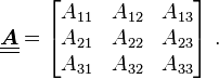
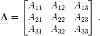
Orthogonal transformations can be represented in Cartesian coordinates by a $3\times 3$ matrix $\underline{\underline{\boldsymbol{A}}}$ given by

\underline{\underline{\boldsymbol{A}}} = \begin{bmatrix} A_{11} & A_{12} & A_{13} \\ A_{21} & A_{22} & A_{23} \\ A_{31} & A_{32} & A_{33} \end{bmatrix}~.

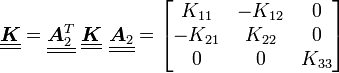
Therefore the symmetry condition can be written in matrix form as

\underline{\underline{\boldsymbol{K}}} = \underline{\underline{\boldsymbol{A}^T}}~\underline{\underline{\boldsymbol{K}}}~\underline{\underline{\boldsymbol{A}}}

Orthotropic material properties

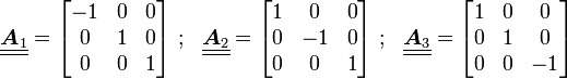
An orthotropic material has three orthogonal symmetry planes. If we choose an orthonormal coordinate system such that the axes coincide with the normals to the three symmetry planes, the transformation matrices are

\underline{\underline{\boldsymbol{A}_1}} = \begin{bmatrix}-1 & 0 & 0 \\ 0 & 1 & 0 \\ 0 & 0 & 1 \end{bmatrix} ~;~~ \underline{\underline{\boldsymbol{A}_2}} = \begin{bmatrix}1 & 0 & 0 \\ 0 & -1 & 0 \\ 0 & 0 & 1 \end{bmatrix} ~;~~ \underline{\underline{\boldsymbol{A}_3}} = \begin{bmatrix}1 & 0 & 0 \\ 0 & 1 & 0 \\ 0 & 0 & -1 \end{bmatrix}

It can be shown that if the matrix $\underline{\underline{\boldsymbol{K}}}$ for a material is invariant under reflection about two orthogonal planes then it is also invariant under reflection about the third orthogonal plane.

Consider the reflection $\underline{\underline{\boldsymbol{A}_3}}$ about the $1-2\,$ plane. Then we have

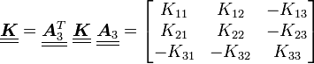
\underline{\underline{\boldsymbol{K}}} = \underline{\underline{\boldsymbol{A}^T_3}}~\underline{\underline{\boldsymbol{K}}}~\underline{\underline{\boldsymbol{A}_3}} = \begin{bmatrix} K_{11} & K_{12} & -K_{13} \\ K_{21} & K_{22} & -K_{23} \\ -K_{31} & -K_{32} & K_{33} \end{bmatrix}

The above relation implies that $K_{13} = K_{23} = K_{31} = K_{32} = 0$ . Next consider a reflection $\underline{\underline{\boldsymbol{A}_2}}$ about the $1-3\,$ plane. We then have

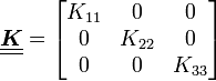
\underline{\underline{\boldsymbol{K}}} = \underline{\underline{\boldsymbol{A}^T_2}}~\underline{\underline{\boldsymbol{K}}}~\underline{\underline{\boldsymbol{A}_2}} = \begin{bmatrix} K_{11} & -K_{12} & 0 \\ -K_{21} & K_{22} & 0 \\ 0 & 0 & K_{33} \end{bmatrix}

That implies that $K_{12} = K_{21} = 0$ . Therefore the material properties of an orthotropic material are described by the matrix

$\underline{\underline{\boldsymbol{K}}} = \begin{bmatrix} K_{11} & 0 & 0 \\ 0 & K_{22} & 0 \\ 0 & 0 & K_{33} \end{bmatrix}$

Orthotropy in linear elasticity

Anisotropic elasticity

In linear elasticity, the relation between stress and strain depend on the type of material under consideration. This relation is known as Hooke's law. For anisotropic materials Hooke's law can be written as^[2]

\boldsymbol{\sigma} = \mathsf{c}\cdot\boldsymbol{\varepsilon}

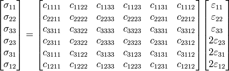
where $\boldsymbol{\sigma}$ is the stress tensor, $\boldsymbol{\varepsilon}$ is the strain tensor, and $\mathsf{c}$ is the elastic stiffness tensor. If the tensors in the above expression are described in terms of components with respect to an orthonormal coordinate system we can write

\sigma_{ij} = c_{ijk\ell}~ \varepsilon_{k\ell}

where summation has been assumed over repeated indices. Since the stress and strain tensors are symmetric, and since the stress-strain relation in linear elasticity can be derived from a strain energy density function, the following symmetries hold for linear elastic materials

c_{ijk\ell} = c_{jik\ell} ~,~~c_{ijk\ell} = c_{ij\ell k} ~,~~ c_{ijk\ell} = c_{k\ell ij} ~.

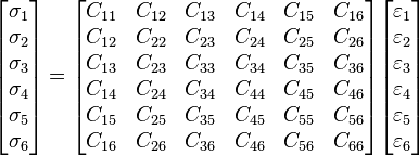
Because of the above symmetries, the stress-strain relation for linear elastic materials can be expressed in matrix form as

\begin{bmatrix}\sigma_{11}\\ \sigma_{22} \\ \sigma_{33} \\ \sigma_{23} \\ \sigma_{31} \\ \sigma_{12} \end{bmatrix} = \begin{bmatrix} c_{1111} & c_{1122} & c_{1133} & c_{1123} & c_{1131} & c_{1112} \\ c_{2211} & c_{2222} & c_{2233} & c_{2223} & c_{2231} & c_{2212} \\ c_{3311} & c_{3322} & c_{3333} & c_{3323} & c_{3331} & c_{3312} \\ c_{2311} & c_{2322} & c_{2333} & c_{2323} & c_{2331} & c_{2312} \\ c_{3111} & c_{3122} & c_{3133} & c_{3123} & c_{3131} & c_{3112} \\ c_{1211} & c_{1222} & c_{1233} & c_{1223} & c_{1231} & c_{1212} \end{bmatrix} \begin{bmatrix}\varepsilon_{11}\\ \varepsilon_{22} \\ \varepsilon_{33} \\ 2\varepsilon_{23} \\ 2\varepsilon_{31} \\ 2\varepsilon_{12} \end{bmatrix}

An alternative representation in Voigt notation is

\begin{bmatrix} \sigma_1 \\ \sigma_2 \\ \sigma_3 \\ \sigma_4 \\ \sigma_5 \\ \sigma_6 \end{bmatrix} = \begin{bmatrix} C_{11} & C_{12} & C_{13} & C_{14} & C_{15} & C_{16} \\ C_{12} & C_{22} & C_{23} & C_{24} & C_{25} & C_{26} \\ C_{13} & C_{23} & C_{33} & C_{34} & C_{35} & C_{36} \\ C_{14} & C_{24} & C_{34} & C_{44} & C_{45} & C_{46} \\ C_{15} & C_{25} & C_{35} & C_{45} & C_{55} & C_{56} \\ C_{16} & C_{26} & C_{36} & C_{46} & C_{56} & C_{66} \end{bmatrix} \begin{bmatrix} \varepsilon_1 \\ \varepsilon_2 \\ \varepsilon_3 \\ \varepsilon_4 \\ \varepsilon_5 \\ \varepsilon_6 \end{bmatrix}

\underline{\underline{\boldsymbol{\sigma}}} = \underline{\underline{\mathsf{C}}}~\underline{\underline{\boldsymbol{\varepsilon}}}

The stiffness matrix $\underline{\underline{\mathsf{C}}}$ in the above relation satisfies point symmetry.^[3]

Condition for material symmetry

The stiffness matrix $\underline{\underline{\mathsf{C}}}$ satisfies a given symmetry condition if it does not change when subjected to the corresponding orthogonal transformation. The orthogonal transformation may represent symmetry with respect to a point, an axis, or a plane. 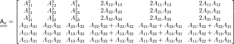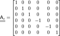Orthogonal transformations in linear elasticity include rotations and reflections, but not shape changing transformations and can be represented, in orthonormal coordinates, by a $3\times 3$ matrix $\underline{\underline{\mathbf{A}}}$ given by

\underline{\underline{\mathbf{A}}} = \begin{bmatrix} A_{11} & A_{12} & A_{13} \\ A_{21} & A_{22} & A_{23} \\ A_{31} & A_{32} & A_{33} \end{bmatrix}~.

In Voigt notation, the transformation matrix for the stress tensor can be expressed as a $6\times6$ matrix $\underline{\underline{\mathsf{A}_\sigma}}$ given by^[3]

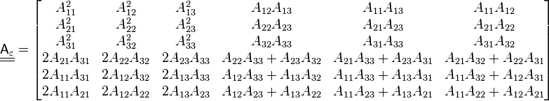
\underline{\underline{\mathsf{A}_\sigma}} = \begin{bmatrix} A_{11}^2 & A_{12}^2 & A_{13}^2 & 2A_{12}A_{13} & 2A_{11}A_{13} & 2A_{11}A_{12} \\ A_{21}^2 & A_{22}^2 & A_{23}^2 & 2A_{22}A_{23} & 2A_{21}A_{23} & 2A_{21}A_{22} \\ A_{31}^2 & A_{32}^2 & A_{33}^2 & 2A_{32}A_{33} & 2A_{31}A_{33} & 2A_{31}A_{32} \\ A_{21}A_{31} & A_{22}A_{32} & A_{23}A_{33} & A_{22}A_{33}+A_{23}A_{32} & A_{21}A_{33}+A_{23}A_{31} & A_{21}A_{32}+A_{22}A_{31} \\ A_{11}A_{31} & A_{12}A_{32} & A_{13}A_{33} & A_{12}A_{33}+A_{13}A_{32} & A_{11}A_{33}+A_{13}A_{31} & A_{11}A_{32}+A_{12}A_{31} \\ A_{11}A_{21} & A_{12}A_{22} & A_{13}A_{23} & A_{12}A_{23}+A_{13}A_{22} & A_{11}A_{23}+A_{13}A_{21} & A_{11}A_{22}+A_{12}A_{21} \end{bmatrix}

The transformation for the strain tensor has a slightly different form because of the choice of notation. This transformation matrix is

\underline{\underline{\mathsf{A}_\varepsilon}} = \begin{bmatrix} A_{11}^2 & A_{12}^2 & A_{13}^2 & A_{12}A_{13} & A_{11}A_{13} & A_{11}A_{12} \\ A_{21}^2 & A_{22}^2 & A_{23}^2 & A_{22}A_{23} & A_{21}A_{23} & A_{21}A_{22} \\ A_{31}^2 & A_{32}^2 & A_{33}^2 & A_{32}A_{33} & A_{31}A_{33} & A_{31}A_{32} \\ 2A_{21}A_{31} & 2A_{22}A_{32} & 2A_{23}A_{33} & A_{22}A_{33}+A_{23}A_{32} & A_{21}A_{33}+A_{23}A_{31} & A_{21}A_{32}+A_{22}A_{31} \\ 2A_{11}A_{31} & 2A_{12}A_{32} & 2A_{13}A_{33} & A_{12}A_{33}+A_{13}A_{32} & A_{11}A_{33}+A_{13}A_{31} & A_{11}A_{32}+A_{12}A_{31} \\ 2A_{11}A_{21} & 2A_{12}A_{22} & 2A_{13}A_{23} & A_{12}A_{23}+A_{13}A_{22} & A_{11}A_{23}+A_{13}A_{21} & A_{11}A_{22}+A_{12}A_{21} \end{bmatrix}

It can be shown that $\underline{\underline{\mathsf{A}_\varepsilon}}^T = \underline{\underline{\mathsf{A}_\sigma}}^{-1}$ .

The elastic properties of a continuum are invariant under an orthogonal transformation $\underline{\underline{\mathbf{A}}}$ if and only if^[3]

$\underline{\underline{\mathsf{C}}} = \underline{\underline{\mathsf{A}_\varepsilon}}^T~\underline{\underline{\mathsf{C}}}~\underline{\underline{\mathsf{A}_\varepsilon}}$

Stiffness and compliance matrices in orthotropic elasticity

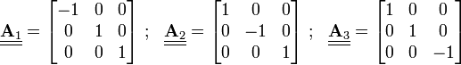
An orthotropic elastic material has three orthogonal symmetry planes. If we choose an orthonormal coordinate system such that the axes coincide with the normals to the three symmetry planes, the transformation matrices are

\underline{\underline{\mathbf{A}_1}} = \begin{bmatrix}-1 & 0 & 0 \\ 0 & 1 & 0 \\ 0 & 0 & 1 \end{bmatrix} ~;~~ \underline{\underline{\mathbf{A}_2}} = \begin{bmatrix}1 & 0 & 0 \\ 0 & -1 & 0 \\ 0 & 0 & 1 \end{bmatrix} ~;~~ \underline{\underline{\mathbf{A}_3}} = \begin{bmatrix}1 & 0 & 0 \\ 0 & 1 & 0 \\ 0 & 0 & -1 \end{bmatrix}

We can show that if the matrix $\underline{\underline{\mathsf{C}}}$ for a linear elastic material is invariant under reflection about two orthogonal planes then it is also invariant under reflection about the third orthogonal plane.

If we consider the reflection $\underline{\underline{\mathbf{A}_3}}$ about the $1-2\,$ plane, then we have

\underline{\underline{\mathsf{A}_\varepsilon}} = \begin{bmatrix} 1 & 0 & 0 & 0 & 0 & 0 \\ 0 & 1 & 0 & 0 & 0 & 0 \\ 0 & 0 & 1 & 0 & 0 & 0 \\ 0 & 0 & 0 & -1 & 0 & 0 \\ 0 & 0 & 0 & 0 & -1 & 0 \\ 0 & 0 & 0 & 0 & 0 & 1 \end{bmatrix}

Then the requirement 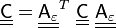$\underline{\underline{\mathsf{C}}} = \underline{\underline{\mathsf{A}_\varepsilon}}^T~\underline{\underline{\mathsf{C}}}~\underline{\underline{\mathsf{A}_\varepsilon}}$ implies that^[3]

\begin{bmatrix} C_{11} & C_{12} & C_{13} & C_{14} & C_{15} & C_{16} \\ C_{12} & C_{22} & C_{23} & C_{24} & C_{25} & C_{26} \\ C_{13} & C_{23} & C_{33} & C_{34} & C_{35} & C_{36} \\ C_{14} & C_{24} & C_{34} & C_{44} & C_{45} & C_{46} \\ C_{15} & C_{25} & C_{35} & C_{45} & C_{55} & C_{56} \\ C_{16} & C_{26} & C_{36} & C_{46} & C_{56} & C_{66} \end{bmatrix} = \begin{bmatrix} C_{11} & C_{12} & C_{13} & -C_{14} & -C_{15} & C_{16} \\ C_{12} & C_{22} & C_{23} & -C_{24} & -C_{25} & C_{26} \\ C_{13} & C_{23} & C_{33} & -C_{34} & -C_{35} & C_{36} \\ -C_{14} & -C_{24} & -C_{34} & C_{44} & C_{45} & -C_{46} \\ -C_{15} & -C_{25} & -C_{35} & C_{45} & C_{55} & -C_{56} \\ C_{16} & C_{26} & C_{36} & -C_{46} & -C_{56} & C_{66} \end{bmatrix}

The above requirement can be satisfied only if

C_{14} = C_{15} = C_{24} = C_{25} = C_{34} = C_{35} = C_{46} = C_{56} = 0 ~.

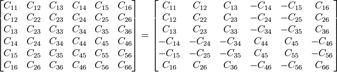
Let us next consider the reflection $\underline{\underline{\mathbf{A}_2}}$ about the $1-3\,$ plane. In that case

\underline{\underline{\mathsf{A}_\varepsilon}} = \begin{bmatrix} 1 & 0 & 0 & 0 & 0 & 0 \\ 0 & 1 & 0 & 0 & 0 & 0 \\ 0 & 0 & 1 & 0 & 0 & 0 \\ 0 & 0 & 0 & -1 & 0 & 0 \\ 0 & 0 & 0 & 0 & 1 & 0 \\ 0 & 0 & 0 & 0 & 0 & -1 \end{bmatrix}

Using the invariance condition again, we get the additional requirement that

C_{16} = C_{26} = C_{36} = C_{45} = 0 ~.

No further information can be obtained because the reflection about third symmetry plane is not independent of reflections about the planes that we have already considered. Therefore, the stiffness matrix of an orthotropic linear elastic material can be written as

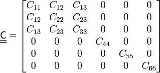
$\underline{\underline{\mathsf{C}}} = \begin{bmatrix} C_{11} & C_{12} & C_{13} & 0 & 0 & 0 \\ C_{12} & C_{22} & C_{23} & 0 & 0 & 0 \\ C_{13} & C_{23} & C_{33} & 0 & 0 & 0 \\ 0 & 0 & 0 & C_{44} & 0 & 0 \\ 0 & 0 & 0 & 0 & C_{55} & 0\\ 0 & 0 & 0 & 0 & 0 & C_{66} \end{bmatrix}$

The inverse of this matrix is commonly written as^[4]

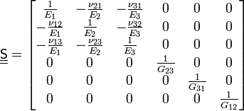
\underline{\underline{\mathsf{S}}} = \begin{bmatrix} \tfrac{1}{E_{\rm 1}} & - \tfrac{\nu_{\rm 21}}{E_{\rm 2}} & - \tfrac{\nu_{\rm 31}}{E_{\rm 3}} & 0 & 0 & 0 \\ -\tfrac{\nu_{\rm 12}}{E_{\rm 1}} & \tfrac{1}{E_{\rm 2}} & - \tfrac{\nu_{\rm 32}}{E_{\rm 3}} & 0 & 0 & 0 \\ -\tfrac{\nu_{\rm 13}}{E_{\rm 1}} & - \tfrac{\nu_{\rm 23}}{E_{\rm 2}} & \tfrac{1}{E_{\rm 3}} & 0 & 0 & 0 \\ 0 & 0 & 0 & \tfrac{1}{G_{\rm 23}} & 0 & 0 \\ 0 & 0 & 0 & 0 & \tfrac{1}{G_{\rm 31}} & 0 \\ 0 & 0 & 0 & 0 & 0 & \tfrac{1}{G_{\rm 12}} \\ \end{bmatrix}

where ${E}_{\rm i}\,$ is the Young's modulus along axis $i$ , $G_{\rm ij}\,$ is the shear modulus in direction $j$ on the plane whose normal is in direction $i$ , and $\nu_{\rm ij}\,$ is the Poisson's ratio that corresponds to a contraction in direction $j$ when an extension is applied in direction $i$ .

Bounds on the moduli of orthotropic elastic materials

The strain-stress relation for orthotropic linear elastic materials can be written in Voigt notation as

\underline{\underline{\boldsymbol{\varepsilon}}} = \underline{\underline{\mathsf{S}}}~\underline{\underline{\boldsymbol{\sigma}}}

where the compliance matrix $\underline{\underline{\mathsf{S}}}$ is given by

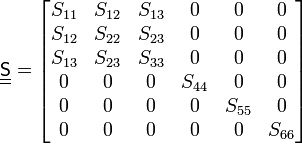
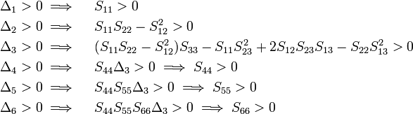
\underline{\underline{\mathsf{S}}} = \begin{bmatrix} S_{11} & S_{12} & S_{13} & 0 & 0 & 0 \\ S_{12} & S_{22} & S_{23} & 0 & 0 & 0 \\ S_{13} & S_{23} & S_{33} & 0 & 0 & 0 \\ 0 & 0 & 0 & S_{44} & 0 & 0 \\ 0 & 0 & 0 & 0 & S_{55} & 0\\ 0 & 0 & 0 & 0 & 0 & S_{66} \end{bmatrix}

The compliance matrix is symmetric and must be positive definite for the strain energy density to be positive. This implies from Sylvester's criterion that all the principal minors of the matrix are positive,^[5] i.e.,

\Delta_k := \det(\underline{\underline{\mathsf{S}_k}}) > 0

where $\underline{\underline{\mathsf{S}_k}}$ is the $k\times k$ principal submatrix of $\underline{\underline{\mathsf{S}}}$ .

Then,

\begin{align} \Delta_1 > 0 & \implies \quad S_{11} > 0 \\ \Delta_2 > 0 & \implies \quad S_{11}S_{22} - S_{12}^2 > 0 \\ \Delta_3 > 0 & \implies \quad (S_{11}S_{22}-S_{12}^2)S_{33}-S_{11}S_{23}^2+2S_{12}S_{23}S_{13}-S_{22}S_{13}^2 >0 \\ \Delta_4 > 0 & \implies \quad S_{44}\Delta_3 > 0 \implies S_{44} > 0\\ \Delta_5 > 0 & \implies \quad S_{44}S_{55}\Delta_3 > 0 \implies S_{55} > 0 \\ \Delta_6 > 0 & \implies \quad S_{44}S_{55}S_{66}\Delta_3 > 0 \implies S_{66} > 0 \end{align}

We can show that this set of conditions implies that^[6]

S_{11} > 0 ~,~~ S_{22} > 0 ~,~~ S_{33} > 0 ~,~~ S_{44} > 0 ~,~~ S_{55} > 0 ~,~~ S_{66} > 0

E_1 > 0 , E_2 > 0, E_3 > 0, G_{12} > 0 , G_{23} > 0, G_{13} > 0

However, no similar lower bounds can be placed on the values of the Poisson's ratios $\nu_{ij}$ .^[5]

References

↑ Milton, G. W., 2002, The Theory of Composites, Cambridge University Press.
↑ Lekhnitskii, S. G., 1963, Theory of Elasticity of an Anisotropic Elastic Body, Holden-Day Inc.
↑ 3.0 3.1 3.2 3.3 Slawinski, M. A., 2010, Waves and Rays in Elastic Continua: 2nd Ed., World Scientific. http://samizdat.mines.edu/wavesandrays/WavesAndRays.pdf
↑ Boresi, A. P, Schmidt, R. J. and Sidebottom, O. M., 1993, Advanced Mechanics of Materials, Wiley.
↑ 5.0 5.1 Ting, T. C. T. and Chen, T., 2005, Poisson's ratio for anisotropic elastic materials can have no bounds,, Q. J. Mech. Appl. Math., 58(1), pp. 73-82.
↑ Ting, T. C. T. (1996), "Positive definiteness of anisotropic elastic constants", Mathematics & Mechanics of Solids 1: 301–314 .

Orthotropic material

Orthotropy in physics

Anisotropic material relations

Condition for material symmetry

Orthotropic material properties

Orthotropy in linear elasticity

Anisotropic elasticity

Condition for material symmetry

Stiffness and compliance matrices in orthotropic elasticity

Bounds on the moduli of orthotropic elastic materials

See also

References

Further reading