Ordinal collapsing function

In mathematical logic and set theory, an ordinal collapsing function (or projection function) is a technique for defining (notations for) certain recursive large countable ordinals, whose principle is to give names to certain ordinals much larger than the one being defined, perhaps even large cardinals (though they can be replaced with recursively large ordinals at the cost of extra technical difficulty), and then “collapse” them down to a system of notations for the sought-after ordinal. For this reason, ordinal collapsing functions are described as an impredicative manner of naming ordinals.

The details of the definition of ordinal collapsing functions vary, and get more complicated as greater ordinals are being defined, but the typical idea is that whenever the notation system “runs out of fuel” and cannot name a certain ordinal, a much larger ordinal is brought “from above” to give a name to that critical point. An example of how this works will be detailed below, for an ordinal collapsing function defining the Bachmann-Howard ordinal (i.e., defining a system of notations up to the Bachmann-Howard ordinal).

The use and definition of ordinal collapsing functions is inextricably intertwined with the theory of ordinal analysis, since the large countable ordinals defined and denoted by a given collapse are used to describe the ordinal-theoretic strength of certain formal systems, typically^[1]^[2] subsystems of analysis (such as those seen in the light of reverse mathematics), extensions of Kripke-Platek set theory, Bishop-style systems of constructive mathematics or Martin-Löf-style systems of intuitionistic type theory.

Ordinal collapsing functions are typically denoted using some variation of the Greek letter $\psi$ (psi).

An example leading up to the Bachmann-Howard ordinal

The choice of the ordinal collapsing function given as example below imitates greatly the system introduced by Buchholz^[3] but is limited to collapsing one cardinal for clarity of exposition. More on the relation between this example and Buchholz's system will be said below.

Definition

Let $\Omega$ stand for the first uncountable ordinal $\omega_1$ , or, in fact, any ordinal which is (an $\varepsilon$ -number and) guaranteed to be greater than all the countable ordinals which will be constructed (for example, the Church-Kleene ordinal is adequate for our purposes; but we will work with $\omega_1$ because it allows the convenient use of the word countable in the definitions).

We define a function $\psi$ (which will be non-decreasing and continuous), taking an arbitrary ordinal $\alpha$ to a countable ordinal $\psi(\alpha)$ , recursively on $\alpha$ , as follows:

Assume

\psi(\beta)

has been defined for all

\beta<\alpha

, and we wish to define

\psi(\alpha)

Let

C(\alpha)

be the set of ordinals generated starting from

0

1

\omega

and

\Omega

by recursively applying the following functions: ordinal addition, multiplication and exponentiation and the function

\psi\upharpoonright_\alpha

, i.e., the restriction of

\psi

to ordinals

\beta<\alpha

. (Formally, we define

C(\alpha)_0 = \{0,1,\omega,\Omega\}

and inductively

C(\alpha)_{n+1} = C(\alpha)_n \cup \{\beta_1+\beta_2,\beta_1\beta_2,{\beta_1}^{\beta_2}: \beta_1,\beta_2\in C(\alpha)_n\} \cup \{\psi(\beta): \beta\in C(\alpha)_n \land \beta<\alpha\}

for all natural numbers

n

and we let

C(\alpha)

be the union of the

C(\alpha)_n

for all

n

Then

\psi(\alpha)

is defined as the smallest ordinal not belonging to

C(\alpha)

In a more concise (although more obscure) way:

\psi(\alpha)

is the smallest ordinal which cannot be expressed from

0

1

\omega

and

\Omega

using sums, products, exponentials, and the

\psi

function itself (to previously constructed ordinals less than

\alpha

Here is an attempt to explain the motivation for the definition of $\psi$ in intuitive terms: since the usual operations of addition, multiplication and exponentiation are not sufficient to designate ordinals very far, we attempt to systematically create new names for ordinals by taking the first one which does not have a name yet, and whenever we run out of names, rather than invent them in an ad hoc fashion or using diagonal schemes, we seek them in the ordinals far beyond the ones we are constructing (beyond $\Omega$ , that is); so we give names to uncountable ordinals and, since in the end the list of names is necessarily countable, $\psi$ will “collapse” them to countable ordinals.

Computation of values of $\psi$

To clarify how the function $\psi$ is able to produce notations for certain ordinals, we now compute its first values.

Predicative start

First consider $C(0)$ . It contains ordinals $0$ , $1$ , $2$ , $3$ , $\omega$ , $\omega+1$ , $\omega+2$ , $\omega2$ , $\omega3$ , $\omega^2$ , $\omega^3$ , $\omega^\omega$ , $\omega^{\omega^\omega}$ and so on. It also contains such ordinals as $\Omega$ , $\Omega+1$ , $\Omega\omega$ , $\Omega^\Omega$ . The first ordinal which it does not contain is $\varepsilon_0$ (which is the limit of $\omega$ , $\omega^\omega$ , $\omega^{\omega^\omega}$ and so on — less than $\Omega$ by assumption). The upper bound of the ordinals it contains is $\varepsilon_{\Omega+1}$ (the limit of $\Omega$ , $\Omega^\Omega$ , $\Omega^{\Omega^\Omega}$ and so on), but that is not so important. This shows that $\psi(0) = \varepsilon_0$ .

Similarly, $C(1)$ contains the ordinals which can be formed from $0$ , $1$ , $\omega$ , $\Omega$ and this time also $\varepsilon_0$ , using addition, multiplication and exponentiation. This contains all the ordinals up to $\varepsilon_1$ but not the latter, so $\psi(1) = \varepsilon_1$ . In this manner, we prove that $\psi(\alpha) = \varepsilon_\alpha$ inductively on $\alpha$ : the proof works, however, only as long as $\alpha<\varepsilon_\alpha$ . We therefore have:

\psi(\alpha) = \varepsilon_\alpha = \phi_1(\alpha)

for all

\alpha\leq\zeta_0

, where

\zeta_0 = \phi_2(0)

is the smallest fixed point of

\alpha \mapsto \varepsilon_\alpha

(Here, the $\phi$ functions are the Veblen functions defined starting with $\phi_1(\alpha) = \varepsilon_\alpha$ .)

Now $\psi(\zeta_0) = \zeta_0$ but $\psi(\zeta_0+1)$ is no larger, since $\zeta_0$ cannot be constructed using finite applications of $\phi_1\colon \alpha\mapsto\varepsilon_\alpha$ and thus never belongs to a $C(\alpha)$ set for $\alpha\leq\Omega$ , and the function $\psi$ remains “stuck” at $\zeta_0$ for some time:

\psi(\alpha) = \zeta_0

for all

\zeta_0 \leq \alpha \leq \Omega

First impredicative values

Again, $\psi(\Omega) = \zeta_0$ . However, when we come to computing $\psi(\Omega+1)$ , something has changed: since $\Omega$ was (“artificially”) added to all the $C(\alpha)$ , we are permitted to take the value $\psi(\Omega) = \zeta_0$ in the process. So $C(\Omega+1)$ contains all ordinals which can be built from $0$ , $1$ , $\omega$ , $\Omega$ , the $\phi_1\colon\alpha\mapsto\varepsilon_\alpha$ function up to $\zeta_0$ and this time also $\zeta_0$ itself, using addition, multiplication and exponentiation. The smallest ordinal not in $C(\Omega+1)$ is $\varepsilon_{\zeta_0+1}$ (the smallest $\varepsilon$ -number after $\zeta_0$ ).

We say that the definition $\psi(\Omega) = \zeta_0$ and the next values of the function $\psi$ such as $\psi(\Omega+1) = \varepsilon_{\zeta_0+1}$ are impredicative because they use ordinals (here, $\Omega$ ) greater than the ones which are being defined (here, $\zeta_0$ ).

Values of $\psi$ up to the Feferman-Schütte ordinal

The fact that $\psi(\Omega+\alpha) = \varepsilon_{\zeta_0+\alpha}$ remains true for all $\alpha \leq \zeta_1 = \phi_2(1)$ (note, in particular, that $\psi(\Omega+\zeta_0) = \varepsilon_{\zeta_0 2}$ : but since now the ordinal $\zeta_0$ has been constructed there is nothing to prevent from going beyond this). However, at $\zeta_1 = \phi_2(1)$ (the first fixed point of $\alpha\mapsto \varepsilon_\alpha$ beyond $\zeta_0$ ), the construction stops again, because $\zeta_1$ cannot be constructed from smaller ordinals and $\zeta_0$ by finitely applying the $\varepsilon$ function. So we have $\psi(\Omega 2) = \zeta_1$ .

The same reasoning shows that $\psi(\Omega(1+\alpha)) = \phi_2(\alpha)$ for all $\alpha\leq\phi_3(0)$ , where $\phi_2$ enumerates the fixed points of $\phi_1\colon\alpha\mapsto\varepsilon_\alpha$ and $\phi_3(0)$ is the first fixed point of $\phi_2$ . We then have $\psi(\Omega^2) = \phi_3(0)$ .

Again, we can see that $\psi(\Omega^\alpha) = \phi_{1+\alpha}(0)$ for some time: this remains true until the first fixed point $\Gamma_0$ of $\alpha \mapsto \phi_\alpha(0)$ , which is the Feferman-Schütte ordinal. Thus, $\psi(\Omega^\Omega) = \Gamma_0$ is the Feferman-Schütte ordinal.

Beyond the Feferman-Schütte ordinal

We have $\psi(\Omega^\Omega+\Omega^\alpha) = \phi_{\Gamma_0+\alpha}(0)$ for all $\alpha\leq\Gamma_1$ where $\Gamma_1$ is the next fixed point of $\alpha \mapsto \phi_\alpha(0)$ . So, if $\alpha\mapsto\Gamma_\alpha$ enumerates the fixed points in question (which can also be noted $\phi(1,0,\alpha)$ using the many-valued Veblen functions) we have $\psi(\Omega^\Omega(1+\alpha)) = \Gamma_\alpha$ , until the first fixed point $\phi(1,1,0)$ of the $\alpha\mapsto\Gamma_\alpha$ itself, which will be $\psi(\Omega^{\Omega+1})$ (and the first fixed point $\phi(2,0,0)$ of the $\alpha \mapsto \phi(1,\alpha,0)$ functions will be $\psi(\Omega^{\Omega2})$ ). In this manner:

$\psi(\Omega^{\Omega^2})$ is the Ackermann ordinal (the range of the notation $\phi(\alpha,\beta,\gamma)$ defined predicatively),
$\psi(\Omega^{\Omega^\omega})$ is the “small” Veblen ordinal (the range of the notations $\phi(\ldots)$ predicatively using finitely many variables),
$\psi(\Omega^{\Omega^\Omega})$ is the “large” Veblen ordinal (the range of the notations $\phi(\ldots)$ predicatively using transfinitely-but-predicatively-many variables),
the limit $\psi(\varepsilon_{\Omega+1})$ of $\psi(\Omega)$ , $\psi(\Omega^\Omega)$ , $\psi(\Omega^{\Omega^\Omega})$ , etc., is the Bachmann-Howard ordinal: after this our function $\psi$ is constant, and we can go no further with the definition we have given.

Ordinal notations up to the Bachmann-Howard ordinal

We now explain more systematically how the $\psi$ function defines notations for ordinals up to the Bachmann-Howard ordinal.

A note about base representations

Recall that if $\delta$ is an ordinal which is a power of $\omega$ (for example $\omega$ itself, or $\varepsilon_0$ , or $\Omega$ ), any ordinal $\alpha$ can be uniquely expressed in the form $\delta^{\beta_1}\gamma_1 + \ldots + \delta^{\beta_k}\gamma_k$ , where $k$ is a natural number, $\gamma_1,\ldots,\gamma_k$ are non-zero ordinals less than $\delta$ , and $\beta_1 > \beta_2 > \cdots > \beta_k$ are ordinal numbers (we allow $\beta_k=0$ ). This “base $\delta$ representation” is an obvious generalization of the Cantor normal form (which is the case $\delta=\omega$ ). Of course, it may quite well be that the expression is uninteresting, i.e., $\alpha = \delta^\alpha$ , but in any other case the $\beta_i$ must all be less than $\alpha$ ; it may also be the case that the expression is trivial (i.e., $\alpha<\delta$ , in which case $k\leq 1$ and $\gamma_1 = \alpha$ ).

If $\alpha$ is an ordinal less than $\varepsilon_{\Omega+1}$ , then its base $\Omega$ representation has coefficients $\gamma_i<\Omega$ (by definition) and exponents $\beta_i<\alpha$ (because of the assumption $\alpha < \varepsilon_{\Omega+1}$ ): hence one can rewrite these exponents in base $\Omega$ and repeat the operation until the process terminates (any decreasing sequence of ordinals is finite). We call the resulting expression the iterated base $\Omega$ representation of $\alpha$ and the various coefficients involved (including as exponents) the pieces of the representation (they are all $<\Omega$ ), or, for short, the $\Omega$ -pieces of $\alpha$ .

Some properties of $\psi$

The function $\psi$ is non-decreasing and continuous (this is more or less obvious from its definition).
If $\psi(\alpha) = \psi(\beta)$ with $\beta<\alpha$ then necessarily $C(\alpha) = C(\beta)$ . Indeed, no ordinal $\beta'$ with $\beta\leq\beta'<\alpha$ can belong to $C(\alpha)$ (otherwise its image by $\psi$ , which is $\psi(\alpha)$ would belong to $C(\alpha)$ — impossible); so $C(\beta)$ is closed by everything under which $C(\alpha)$ is the closure, so they are equal.
Any value $\gamma=\psi(\alpha)$ taken by $\psi$ is an $\varepsilon$ -number (i.e., a fixed point of $\beta\mapsto\omega^\beta$ ). Indeed, if it were not, then by writing it in Cantor normal form, it could be expressed using sums, products and exponentiation from elements less than it, hence in $C(\alpha)$ , so it would be in $C(\alpha)$ , a contradiction.
Lemma: Assume $\delta$ is an $\varepsilon$ -number and $\alpha$ an ordinal such that $\psi(\beta)<\delta$ for all $\beta<\alpha$ : then the $\Omega$ -pieces (defined above) of any element of $C(\alpha)$ are less than $\delta$ . Indeed, let $C'$ be the set of ordinals all of whose $\Omega$ -pieces are less than $\delta$ . Then $C'$ is closed under addition, multiplication and exponentiation (because $\delta$ is an $\varepsilon$ -number, so ordinals less than it are closed under addition, multiplication and exponentiation). And $C'$ also contains every $\psi(\beta)$ for $\beta<\alpha$ by assumption, and it contains $0$ , $1$ , $\omega$ , $\Omega$ . So $C'\supseteq C(\alpha)$ , which was to be shown.
Under the hypothesis of the previous lemma, $\psi(\alpha) \leq \delta$ (indeed, the lemma shows that $\delta \not\in C(\alpha)$ ).
Any $\varepsilon$ -number less than some element in the range of $\psi$ is itself in the range of $\psi$ (that is, $\psi$ omits no $\varepsilon$ -number). Indeed: if $\delta$ is an $\varepsilon$ -number not greater than the range of $\psi$ , let $\alpha$ be the least upper bound of the $\beta$ such that $\psi(\beta)<\delta$ : then by the above we have $\psi(\alpha)\leq\delta$ , but $\psi(\alpha)<\delta$ would contradict the fact that $\alpha$ is the least upper bound — so $\psi(\alpha)=\delta$ .
Whenever $\psi(\alpha) = \delta$ , the set $C(\alpha)$ consists exactly of those ordinals $\gamma$ (less than $\varepsilon_{\Omega+1}$ ) all of whose $\Omega$ -pieces are less than $\delta$ . Indeed, we know that all ordinals less than $\delta$ , hence all ordinals (less than $\varepsilon_{\Omega+1}$ ) whose $\Omega$ -pieces are less than $\delta$ , are in $C(\alpha)$ . Conversely, if we assume $\psi(\beta) < \delta$ for all $\beta<\alpha$ (in other words if $\alpha$ is the least possible with $\psi(\alpha)=\delta$ ), the lemma gives the desired property. On the other hand, if $\psi(\alpha) = \psi(\beta)$ for some $\beta<\alpha$ , then we have already remarked $C(\alpha) = C(\beta)$ and we can replace $\alpha$ by the least possible with $\psi(\alpha)=\delta$ .

The ordinal notation

Using the facts above, we can define a (canonical) ordinal notation for every $\gamma$ less than the Bachmann-Howard ordinal. We do this by induction on $\gamma$ .

If $\gamma$ is less than $\varepsilon_0$ , we use the iterated Cantor normal form of $\gamma$ . Otherwise, there exists a largest $\varepsilon$ -number $\delta$ less or equal to $\gamma$ (this is because the set of $\varepsilon$ -numbers is closed): if $\delta<\gamma$ then by induction we have defined a notation for $\delta$ and the base $\delta$ representation of $\gamma$ gives one for $\gamma$ , so we are finished.

It remains to deal with the case where $\gamma=\delta$ is an $\varepsilon$ -number: we have argued that, in this case, we can write $\delta = \psi(\alpha)$ for some (possibly uncountable) ordinal $\alpha<\varepsilon_{\Omega+1}$ : let $\alpha$ be the greatest possible such ordinal (which exists since $\psi$ is continuous). We use the iterated base $\Omega$ representation of $\alpha$ : it remains to show that every piece of this representation is less than $\delta$ (so we have already defined a notation for it). If this is not the case then, by the properties we have shown, $C(\alpha)$ does not contain $\alpha$ ; but then $C(\alpha+1)=C(\alpha)$ (they are closed under the same operations, since the value of $\psi$ at $\alpha$ can never be taken), so $\psi(\alpha+1)=\psi(\alpha)=\delta$ , contradicting the maximality of $\alpha$ .

Note: Actually, we have defined canonical notations not just for ordinals below the Bachmann-Howard ordinal but also for certain uncountable ordinals, namely those whose $\Omega$ -pieces are less than the Bachmann-Howard ordinal (viz.: write them in iterated base $\Omega$ representation and use the canonical representation for every piece). This canonical notation is used for arguments of the $\psi$ function (which may be uncountable).

Examples

For ordinals less than $\varepsilon_0 = \psi(0)$ , the canonical ordinal notation defined coincides with the iterated Cantor normal form (by definition).

For ordinals less than $\varepsilon_1 = \psi(1)$ , the notation coincides with iterated base $\varepsilon_0$ notation (the pieces being themselves written in iterated Cantor normal form): e.g., $\omega^{\omega^{\varepsilon_0+\omega}}$ will be written ${\varepsilon_0}^{\omega^\omega}$ , or, more accurately, $\psi(0)^{\omega^\omega}$ . For ordinals less than $\varepsilon_2 = \psi(2)$ , we similarly write in iterated base $\varepsilon_1$ and then write the pieces in iterated base $\varepsilon_0$ (and write the pieces of that in iterated Cantor normal form): so $\omega^{\omega^{\varepsilon_1+\varepsilon_0+1}}$ is written ${\varepsilon_1}^{\varepsilon_0\omega}$ , or, more accurately, $\psi(1)^{\psi(0)\,\omega}$ . Thus, up to $\zeta_0 = \psi(\Omega)$ , we always use the largest possible $\varepsilon$ -number base which gives a non-trivial representation.

Beyond this, we may need to express ordinals beyond $\Omega$ : this is always done in iterated $\Omega$ -base, and the pieces themselves need to be expressed using the largest possible $\varepsilon$ -number base which gives a non-trivial representation.

Note that while $\psi(\varepsilon_{\Omega+1})$ is equal to the Bachmann-Howard ordinal, this is not a “canonical notation” in the sense we have defined (canonical notations are defined only for ordinals less than the Bachmann-Howard ordinal).

Conditions for canonicalness

The notations thus defined have the property that whenever they nest $\psi$ functions, the arguments of the “inner” $\psi$ function are always less than those of the “outer” one (this is a consequence of the fact that the $\Omega$ -pieces of $\alpha$ , where $\alpha$ is the largest possible such that $\psi(\alpha)=\delta$ for some $\varepsilon$ -number $\delta$ , are all less than $\delta$ , as we have shown above). For example, $\psi(\psi(\Omega)+1)$ does not occur as a notation: it is a well-defined expression (and it is equal to $\psi(\Omega) = \zeta_0$ since $\psi$ is constant between $\zeta_0$ and $\Omega$ ), but it is not a notation produced by the inductive algorithm we have outlined.

Canonicalness can be checked recursively: an expression is canonical if and only if it is either the iterated Cantor normal form of an ordinal less than $\varepsilon_0$ , or an iterated base $\delta$ representation all of whose pieces are canonical, for some $\delta=\psi(\alpha)$ where $\alpha$ is itself written in iterated base $\Omega$ representation all of whose pieces are canonical and less than $\delta$ . The order is checked by lexicographic verification at all levels (keeping in mind that $\Omega$ is greater than any expression obtained by $\psi$ , and for canonical values the greater $\psi$ always trumps the lesser or even arbitrary sums, products and exponentials of the lesser).

For example, $\psi(\Omega^{\omega+1}\,\psi(\Omega) + \psi(\Omega^\omega)^{\psi(\Omega^2)}42)^{\psi(1729)\,\omega}$ is a canonical notation for an ordinal which is less than the Feferman-Schütte ordinal: it can be written using the Veblen functions as $\phi_1(\phi_{\omega+1}(\phi_2(0)) + \phi_\omega(0)^{\phi_3(0)}42)^{\phi_1(1729)\,\omega}$ .

Concerning the order, one might point out that $\psi(\Omega^\Omega)$ (the Feferman-Schütte ordinal) is much more than $\psi(\Omega^{\psi(\Omega)}) = \phi_{\phi_2(0)}(0)$ (because $\Omega$ is greater than $\psi$ of anything), and $\psi(\Omega^{\psi(\Omega)}) = \phi_{\phi_2(0)}(0)$ is itself much more than $\psi(\Omega)^{\psi(\Omega)} = \phi_2(0)^{\phi_2(0)}$ (because $\Omega^{\psi(\Omega)}$ is greater than $\Omega$ , so any sum-product-or-exponential expression involving $\psi(\Omega)$ and smaller value will remain less than $\psi(\Omega^\Omega)$ ). In fact, $\psi(\Omega)^{\psi(\Omega)}$ is already less than $\psi(\Omega+1)$ .

Standard sequences for ordinal notations

To witness the fact that we have defined notations for ordinals below the Bachmann-Howard ordinal (which are all of countable cofinality), we might define standard sequences converging to any one of them (provided it is a limit ordinal, of course). Actually we will define canonical sequences for certain uncountable ordinals, too, namely the uncountable ordinals of countable cofinality (if we are to hope to define a sequence converging to them…) which are representable (that is, all of whose $\Omega$ -pieces are less than the Bachmann-Howard ordinal).

The following rules are more or less obvious, except for the last:

First, get rid of the (iterated) base representations: to define a standard sequence converging to , where is either or (or , but see below):
- if $k$ is zero then $\alpha=0$ and there is nothing to be done;
- if $\beta_k$ is zero and $\gamma_k$ is successor, then $\alpha$ is successor and there is nothing to be done;
- if $\gamma_k$ is limit, take the standard sequence converging to $\gamma_k$ and replace $\gamma_k$ in the expression by the elements of that sequence;
- if $\gamma_k$ is successor and $\beta_k$ is limit, rewrite the last term $\delta^{\beta_k}\gamma_k$ as $\delta^{\beta_k}(\gamma_k-1) + \delta^{\beta_k}$ and replace the exponent $\beta_k$ in the last term by the elements of the fundamental sequence converging to it;
- if $\gamma_k$ is successor and $\beta_k$ is also, rewrite the last term $\delta^{\beta_k}\gamma_k$ as $\delta^{\beta_k}(\gamma_k-1) + \delta^{\beta_k-1}\delta$ and replace the last $\delta$ in this expression by the elements of the fundamental sequence converging to it.
If $\delta$ is $\omega$ , then take the obvious $0$ , $1$ , $2$ , $3$ … as the fundamental sequence for $\delta$ .
If $\delta = \psi(0)$ then take as fundamental sequence for $\delta$ the sequence $\omega$ , $\omega^\omega$ , $\omega^{\omega^\omega}$ …
If $\delta = \psi(\alpha+1)$ then take as fundamental sequence for $\delta$ the sequence $\psi(\alpha)$ , $\psi(\alpha)^{\psi(\alpha)}$ , $\psi(\alpha)^{\psi(\alpha)^{\psi(\alpha)}}$ …
If $\delta = \psi(\alpha)$ where $\alpha$ is a limit ordinal of countable cofinality, define the standard sequence for $\delta$ to be obtained by applying $\psi$ to the standard sequence for $\alpha$ (recall that $\psi$ is continuous, here).
It remains to handle the case where $\delta = \psi(\alpha)$ with $\alpha$ an ordinal of uncountable cofinality (e.g., $\Omega$ itself). Obviously it doesn't make sense to define a sequence converging to $\alpha$ in this case; however, what we can define is a sequence converging to some $\rho<\alpha$ with countable cofinality and such that $\psi$ is constant between $\rho$ and $\alpha$ . This $\rho$ will be the first fixed point of a certain (continuous and non-decreasing) function $\xi\mapsto h(\psi(\xi))$ . To find it, apply the same rules (from the base $\Omega$ representation of $\alpha$ ) as to find the canonical sequence of $\alpha$ , except that whenever a sequence converging to $\Omega$ is called for (something which cannot exist), replace the $\Omega$ in question, in the expression of $\alpha = h(\Omega)$ , by a $\psi(\xi)$ (where $\xi$ is a variable) and perform a repeated iteration (starting from $0$ , say) of the function $\xi\mapsto h(\psi(\xi))$ : this gives a sequence $0$ , $h(\psi(0))$ , $h(\psi(h(\psi(0))))$ … tending to $\rho$ , and the canonical sequence for $\psi(\alpha) = \psi(\rho)$ is $\psi(0)$ , $\psi(h(\psi(0)))$ , $\psi(h(\psi(h(\psi(0)))))$ … (The examples below should make this clearer.)

Here are some examples for the last (and most interesting) case:

The canonical sequence for $\psi(\Omega)$ is: $\psi(0)$ , $\psi(\psi(0))$ , $\psi(\psi(\psi(0)))$ … This indeed converges to $\rho = \psi(\Omega) = \zeta_0$ after which $\psi$ is constant until $\Omega$ .
The canonical sequence for $\psi(\Omega 2)$ is: $\psi(0)$ , $\psi(\Omega+\psi(0))$ , $\psi(\Omega+\psi(\Omega+\psi(0)))$ … This indeed converges to the value of $\psi$ at $\rho = \Omega + \psi(\Omega 2) = \Omega + \zeta_1$ after which $\psi$ is constant until $\Omega 2$ .
The canonical sequence for $\psi(\Omega^2)$ is: $\psi(0)$ , $\psi(\Omega\psi(0))$ , $\psi(\Omega\psi(\Omega\psi(0)))$ … This converges to the value of $\psi$ at $\rho = \Omega \psi(\Omega^2)$ .
The canonical sequence for $\psi(\Omega^2 3 + \Omega)$ is $\psi(0)$ , $\psi(\Omega^2 3 + \psi(0))$ , $\psi(\Omega^2 3 + \psi(\Omega^2 3 + \psi(0)))$ … This converges to the value of $\psi$ at $\rho = \Omega^2 3 + \psi(\Omega^2 3 + \Omega)$ .
The canonical sequence for $\psi(\Omega^\Omega)$ is: $\psi(0)$ , $\psi(\Omega^{\psi(0)})$ , $\psi(\Omega^{\psi(\Omega^{\psi(0)})})$ … This converges to the value of $\psi$ at $\rho = \Omega^{\psi(\Omega^\Omega)}$ .
The canonical sequence for $\psi(\Omega^\Omega 3)$ is: $\psi(0)$ , $\psi(\Omega^\Omega 2+\Omega^{\psi(0)})$ , $\psi(\Omega^\Omega 2+\Omega^{\psi(\Omega^\Omega 2+\Omega^{\psi(0)})})$ … This converges to the value of $\psi$ at $\rho = \Omega^\Omega 2 + \Omega^{\psi(\Omega^\Omega 3)}$ .
The canonical sequence for $\psi(\Omega^{\Omega+1})$ is: $\psi(0)$ , $\psi(\Omega^\Omega \psi(0))$ , $\psi(\Omega^\Omega \psi(\Omega^\Omega \psi(0)))$ … This converges to the value of $\psi$ at $\rho = \Omega^\Omega \psi(\Omega^{\Omega+1})$ .
The canonical sequence for $\psi(\Omega^{\Omega^2+\Omega 3})$ is: $\psi(0)$ , $\psi(\Omega^{\Omega^2+\Omega 2+\psi(0)})$ , $\psi(\Omega^{\Omega^2+\Omega 2+\psi(\Omega^{\Omega^2+\Omega 2+\psi(0)})})$ …

Here are some examples of the other cases:

The canonical sequence for $\omega^2$ is: $0$ , $\omega$ , $\omega 2$ , $\omega 3$ …
The canonical sequence for $\psi(\omega^\omega)$ is: $\psi(1)$ , $\psi(\omega)$ , $\psi(\omega^2)$ , $\psi(\omega^3)$ …
The canonical sequence for $\psi(\Omega)^\omega$ is: $1$ , $\psi(\Omega)$ , $\psi(\Omega)^2$ , $\psi(\Omega)^3$ …
The canonical sequence for $\psi(\Omega+1)$ is: $\psi(\Omega)$ , $\psi(\Omega)^{\psi(\Omega)}$ , $\psi(\Omega)^{\psi(\Omega)^{\psi(\Omega)}}$ …
The canonical sequence for $\psi(\Omega+\omega)$ is: $\psi(\Omega)$ , $\psi(\Omega+1)$ , $\psi(\Omega+2)$ , $\psi(\Omega+3)$ …
The canonical sequence for $\psi(\Omega\omega)$ is: $\psi(0)$ , $\psi(\Omega)$ , $\psi(\Omega 2)$ , $\psi(\Omega 3)$ …
The canonical sequence for $\psi(\Omega^\omega)$ is: $\psi(1)$ , $\psi(\Omega)$ , $\psi(\Omega^2)$ , $\psi(\Omega^3)$ …
The canonical sequence for $\psi(\Omega^{\psi(0)})$ is: $\psi(\Omega^\omega)$ , $\psi(\Omega^{\omega^\omega})$ , $\psi(\Omega^{\omega^{\omega^\omega}})$ … (this is derived from the fundamental sequence for $\psi(0)$ ).
The canonical sequence for $\psi(\Omega^{\psi(\Omega)})$ is: $\psi(\Omega^{\psi(0)})$ , $\psi(\Omega^{\psi(\psi(0))})$ , $\psi(\Omega^{\psi(\psi(\psi(0)))})$ … (this is derived from the fundamental sequence for $\psi(\Omega)$ , which was given above).

Even though the Bachmann-Howard ordinal $\psi(\varepsilon_{\Omega+1})$ itself has no canonical notation, it is also useful to define a canonical sequence for it: this is $\psi(\Omega)$ , $\psi(\Omega^\Omega)$ , $\psi(\Omega^{\Omega^\Omega})$ …

A terminating process

Start with any ordinal less or equal to the Bachmann-Howard ordinal, and repeat the following process so long as it is not zero:

if the ordinal is a successor, subtract one (that is, replace it with its predecessor),
if it is a limit, replace it by some element of the canonical sequence defined for it.

Then it is true that this process always terminates (as any decreasing sequence of ordinals is finite); however, like (but even more so than for) the hydra game:

it can take a very long time to terminate,
the proof of termination may be out of reach of certain weak systems of arithmetic.

To give some flavor of what the process feels like, here are some steps of it: starting from $\psi(\Omega^{\Omega^\omega})$ (the small Veblen ordinal), we might go down to $\psi(\Omega^{\Omega^3})$ , from there down to $\psi(\Omega^{\Omega^2 \psi(0)})$ , then $\psi(\Omega^{\Omega^2 \omega^\omega})$ then $\psi(\Omega^{\Omega^2 \omega^3})$ then $\psi(\Omega^{\Omega^2 \omega^2 7})$ then $\psi(\Omega^{\Omega^2 (\omega^2 6 + \omega)})$ then $\psi(\Omega^{\Omega^2 (\omega^2 6 + 1)})$ then $\psi(\Omega^{\Omega^2 \omega^2 6 + \Omega \psi(\Omega^{\Omega^2 \omega^2 6 + \Omega \psi(0)})})$ and so on. It appears as though the expressions are getting more and more complicated whereas, in fact, the ordinals always decrease.

Concerning the first statement, one could introduce, for any ordinal $\alpha$ less or equal to the Bachmann-Howard ordinal $\psi(\varepsilon_{\Omega+1})$ , the integer function $f_\alpha(n)$ which counts the number of steps of the process before termination if one always selects the $n$ 'th element from the canonical sequence. Then $f_\alpha$ can be a very fast growing function: already $f_{\omega^\omega}(n)$ is essentially $n^n$ , the function $f_{\psi(\Omega^\omega)}(n)$ is comparable with the Ackermann function $A(n,n)$ , and $f_{\psi(\varepsilon_{\Omega+1})}(n)$ is quite unimaginable.

Concerning the second statement, a precise version is given by ordinal analysis: for example, Kripke-Platek set theory can prove^[4] that the process terminates for any given $\alpha$ less than the Bachmann-Howard ordinal, but it cannot do this uniformly, i.e., it cannot prove the termination starting from the Bachmann-Howard ordinal. Some theories like Peano arithmetic are limited by much smaller ordinals ( $\varepsilon_0$ in the case of Peano arithmetic).

Variations on the example

Making the function less powerful

It is instructive (although not exactly useful) to make $\psi$ less powerful.

If we alter the definition of $\psi$ above to omit exponentiation from the repertoire from which $C(\alpha)$ is constructed, then we get $\psi(0) = \omega^\omega$ (as this is the smallest ordinal which cannot be constructed from $0$ , $1$ and $\omega$ using addition and multiplication only), then $\psi(1) = \omega^{\omega^2}$ and similarly $\psi(\omega) = \omega^{\omega^\omega}$ , $\psi(\psi(0)) = \omega^{\omega^{\omega^\omega}}$ until we come to a fixed point which is then our $\psi(\Omega) = \varepsilon_0$ . We then have $\psi(\Omega+1) = {\varepsilon_0}^\omega$ and so on until $\psi(\Omega 2) = \varepsilon_1$ . Since multiplication of $\Omega$ 's is permitted, we can still form $\psi(\Omega^2) = \phi_2(0)$ and $\psi(\Omega^3) = \phi_3(0)$ and so on, but our construction ends there as there is no way to get at or beyond $\Omega^\omega$ : so the range of this weakened system of notation is $\psi(\Omega^\omega) = \phi_\omega(0)$ (the value of $\psi(\Omega^\omega)$ is the same in our weaker system as in our original system, except that now we cannot go beyond it). This does not even go as far as the Feferman-Schütte ordinal.

If we alter the definition of $\psi$ yet some more to allow only addition as a primitive for construction, we get $\psi(0) = \omega^2$ and $\psi(1) = \omega^3$ and so on until $\psi(\psi(0)) = \omega^{\omega^2}$ and still $\psi(\Omega) = \varepsilon_0$ . This time, $\psi(\Omega+1) = \varepsilon_0 \omega$ and so on until $\psi(\Omega 2) = \varepsilon_1$ and similarly $\psi(\Omega 3) = \varepsilon_2$ . But this time we can go no further: since we can only add $\Omega$ 's, the range of our system is $\psi(\Omega\omega) = \varepsilon_\omega = \phi_1(\omega)$ .

In both cases, we find that the limitation on the weakened $\psi$ function comes not so much from the operations allowed on the countable ordinals as on the uncountable ordinals we allow ourselves to denote.

Going beyond the Bachmann-Howard ordinal

We know that $\psi(\varepsilon_{\Omega+1})$ is the Bachmann-Howard ordinal. The reason why $\psi(\varepsilon_{\Omega+1}+1)$ is no larger, with our definitions, is that there is no notation for $\varepsilon_{\Omega+1}$ (it does not belong to $C(\alpha)$ for any $\alpha$ , it is always the least upper bound of it). One could try to add the $\varepsilon$ function (or the Veblen functions of so-many-variables) to the allowed primitives beyond addition, multiplication and exponentiation, but that does not get us very far. To create more systematic notations for countable ordinals, we need more systematic notations for uncountable ordinals: we cannot use the $\psi$ function itself because it only yields countable ordinals (e.g., $\psi(\Omega+1)$ is, $\varepsilon_{\phi_2(0)+1}$ , certainly not $\varepsilon_{\Omega+1}$ ), so the idea is to mimic its definition as follows:

Let

\psi_1(\alpha)

be the smallest ordinal which cannot be expressed from all countable ordinals,

\Omega

and

\Omega_2

using sums, products, exponentials, and the

\psi_1

function itself (to previously constructed ordinals less than

\alpha

Here, $\Omega_2$ is a new ordinal guaranteed to be greater than all the ordinals which will be constructed using $\psi_1$ : again, letting $\Omega = \omega_1$ and $\Omega_2 = \omega_2$ works.

For example, $\psi_1(0) = \varepsilon_{\Omega+1}$ , and more generally $\psi_1(\alpha) = \varepsilon_{\Omega+1+\alpha}$ for all countable ordinals and even beyond ( $\psi_1(\Omega) = \varepsilon_{\Omega 2}$ and $\psi_1(\psi_1(0)) = \varepsilon_{\Omega+\varepsilon_{\Omega+1}}$ ): this holds up to the first fixed point $\zeta_{\Omega+1}$ beyond $\Omega$ of the $\xi\mapsto\varepsilon_\xi$ function, which is the limit of $\psi_1(0)$ , $\psi_1(\psi_1(0))$ and so forth. Beyond this, we have $\psi_1(\alpha) = \zeta_{\Omega+1}$ and this remains true until $\Omega_2$ : exactly as was the case for $\psi(\Omega)$ , we have $\psi_1(\Omega_2) = \zeta_{\Omega+1}$ and $\psi_1(\Omega_2+1) = \varepsilon_{\zeta_{\Omega+1}+1}$ .

The $\psi_1$ function gives us a system of notations (assuming we can somehow write down all countable ordinals!) for the uncountable ordinals below $\psi_1(\varepsilon_{\Omega_2+1})$ , which is the limit of $\psi_1(\Omega_2)$ , $\psi_1({\Omega_2}^{\Omega_2})$ and so forth.

Now we can reinject these notations in the original $\psi$ function, modified as follows:

\psi(\alpha)

is the smallest ordinal which cannot be expressed from

0

1

\omega

\Omega

and

\Omega_2

using sums, products, exponentials, the

\psi_1

function, and the

\psi

function itself (to previously constructed ordinals less than

\alpha

This modified function $\psi$ coincides with the previous one up to (and including) $\psi(\psi_1(0))$ — which is the Bachmann-Howard ordinal. But now we can get beyond this, and $\psi(\psi_1(0)+1)$ is $\varepsilon_{\psi(\psi_1(0))+1}$ (the next $\varepsilon$ -number after the Bachmann-Howard ordinal). We have made our system doubly impredicative: to create notations for countable ordinals we use notations for certain ordinals between $\Omega$ and $\Omega_2$ which are themselves defined using certain ordinals beyond $\Omega_2$ .

A variation on this scheme, which makes little difference when using just two (or finitely many) collapsing functions, but becomes important for infinitely many of them, is to define

\psi(\alpha)

is the smallest ordinal which cannot be expressed from

0

1

\omega

\Omega

and

\Omega_2

using sums, products, exponentials, and the

\psi_1

and

\psi

function (to previously constructed ordinals less than

\alpha

i.e., allow the use of $\psi_1$ only for arguments less than $\alpha$ itself. With this definition, we must write $\psi(\Omega_2)$ instead of $\psi(\psi_1(\Omega_2))$ (although it is still also equal to $\psi(\psi_1(\Omega_2)) = \psi(\zeta_{\Omega+1})$ , of course, but it is now constant until $\Omega_2$ ). This change is inessential because, intuitively speaking, the $\psi_1$ function collapses the nameable ordinals beyond $\Omega_2$ below the latter so it matters little whether $\psi$ is invoked directly on the ordinals beyond $\Omega_2$ or on their image by $\psi_1$ . But it makes it possible to define $\psi$ and $\psi_1$ by simultaneous (rather than “downward”) induction, and this is important if we are to use infinitely many collapsing functions.

Indeed, there is no reason to stop at two levels: using $\omega+1$ new cardinals in this way, $\Omega_1,\Omega_2,\ldots,\Omega_\omega$ , we get a system essentially equivalent to that introduced by Buchholz,^[3] the inessential difference being that since Buchholz uses $\omega+1$ ordinals from the start, he does not need to allow multiplication or exponentiation; also, Buchholz does not introduce the numbers $1$ or $\omega$ in the system as they will also be produced by the $\psi$ functions: this makes the entire scheme much more elegant and more concise to define, albeit more difficult to understand. This system is also sensibly equivalent to the earlier (and much more difficult to grasp) “ordinal diagrams” of Takeuti^[5] and $\theta$ functions of Feferman: their range is the same ( $\psi_0(\varepsilon_{\Omega_\omega+1})$ , which could be called the Takeuti-Feferman-Buchholz ordinal, and which describes the strength of $\Pi^1_1$ -comprehension plus bar induction).

A "normal" variant

Most definitions of ordinal collapsing functions found in the recent literature differ from the ones we have given in one technical but important way which makes them technically more convenient although intuitively less transparent. We now explain this.

The following definition (by induction on $\alpha$ ) is completely equivalent to that of the function $\psi$ above:

Let

C(\alpha,\beta)

be the set of ordinals generated starting from

0

1

\omega

\Omega

and all ordinals less than

\beta

by recursively applying the following functions: ordinal addition, multiplication and exponentiation, and the function

\psi\upharpoonright_\alpha

. Then

\psi(\alpha)

is defined as the smallest ordinal

\rho

such that

C(\alpha,\rho) \cap \Omega = \rho

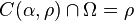(This is equivalent, because if $\sigma$ is the smallest ordinal not in $C(\alpha,0)$ , which is how we originally defined $\psi(\alpha)$ , then it is also the smallest ordinal not in 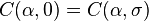$C(\alpha,0) = C(\alpha,\sigma)$ , and furthermore the properties we described of $\psi$ imply that no ordinal between $\sigma$ inclusive and $\Omega$ exclusive belongs to $C(\alpha,\sigma)$ .)

We can now make a change to the definition which makes it subtly different:

Let

\tilde C(\alpha,\beta)

be the set of ordinals generated starting from

0

1

\omega

\Omega

and all ordinals less than

\beta

by recursively applying the following functions: ordinal addition, multiplication and exponentiation, and the function

\tilde\psi\upharpoonright_\alpha

. Then

\tilde\psi(\alpha)

is defined as the smallest ordinal

\rho

such that

\tilde C(\alpha,\rho) \cap \Omega = \rho

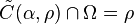and

\alpha \in \tilde C(\alpha,\rho)

The first values of $\tilde\psi$ coincide with those of $\psi$ : namely, for all $\alpha<\zeta_0$ where $\zeta_0 = \varphi_2(0)$ , we have $\tilde\psi(\alpha) = \psi(\alpha)$ because the additional clause $\alpha \in \tilde C(\alpha,\rho)$ is always satisfied. But at this point the functions start to differ: while the function $\psi$ gets “stuck” at $\zeta_0$ for all $\zeta_0 \leq \alpha \leq \Omega$ , the function $\tilde\psi$ satisfies $\tilde\psi(\zeta_0) = \varepsilon_{\zeta_0+1}$ because the new condition $\alpha \in \tilde C(\alpha,\rho)$ imposes $\tilde\psi(\zeta_0) > \zeta_0$ . On the other hand, we still have $\tilde\psi(\Omega) = \zeta_0$ (because $\Omega \in C(\alpha,\rho)$ for all $\rho$ so the extra condition does not come in play). Note in particular that $\tilde\psi$ , unlike $\psi$ , is not monotonic, nor is it continuous.

Despite these changes, the $\tilde\psi$ function also defines a system of ordinal notations up to the Bachmann-Howard ordinal: the notations, and the conditions for canonicalness, are slightly different (for example, $\psi(\Omega+1+\alpha) = \tilde\psi(\tilde\psi(\Omega)+\alpha)$ for all $\alpha$ less than the common value $\psi(\Omega2) = \tilde\psi(\Omega+1)$ ).

Collapsing large cardinals

As noted in the introduction, the use and definition of ordinal collapsing functions is strongly connected with the theory of ordinal analysis, so the collapse of this or that large cardinal must be mentioned simultaneously with the theory for which it provides a proof-theoretic analysis.

Gerhard Jäger and Wolfram Pohlers^[6] described the collapse of an inaccessible cardinal to describe the ordinal-theoretic strength of Kripke-Platek set theory augmented by the recursive inaccessibility of the class of ordinals (KPi), which is also proof-theoretically equivalent^[1] to $\Delta^1_2$ -comprehension plus bar induction. Roughly speaking, this collapse can be obtained by adding the $\alpha \mapsto \Omega_\alpha$ function itself to the list of constructions to which the $C(\cdot)$ collapsing system applies.
Michael Rathjen^[7] then described the collapse of a Mahlo cardinal to describe the ordinal-theoretic strength of Kripke-Platek set theory augmented by the recursive mahloness of the class of ordinals (KPM).
The same author^[8] later described the collapse of a weakly compact cardinal to describe the ordinal-theoretic strength of Kripke-Platek set theory augmented by certain reflection principles (concentrating on the case of $\Pi_3$ -reflection). Very roughly speaking, this proceeds by introducing the first cardinal $\Xi(\alpha)$ which is $\alpha$ -hyper-Mahlo and adding the $\alpha \mapsto \Xi(\alpha)$ function itself to the collapsing system.
Even more recently, the same author has begun^[9] the investigation of the collapse of yet larger cardinals, with the ultimate goal of achieving an ordinal analysis of $\Pi^1_2$ -comprehension (which is proof-theoretically equivalent to the augmentation of Kripke-Platek by $\Sigma_1$ -separation).

Notes

↑ 1.0 1.1 Rathjen, 1995 (Bull. Symbolic Logic)
↑ Kahle, 2002 (Synthese)
↑ 3.0 3.1 Buchholz, 1986 (Ann. Pure Appl. Logic)
↑ Rathjen, 2005 (Fischbachau slides)
↑ Takeuti, 1967 (Ann. Math.)
↑ Jäger & Pohlers, 1983 (Bayer. Akad. Wiss. Math.-Natur. Kl. Sitzungsber.)
↑ Rathjen, 1991 (Arch. Math. Logic)
↑ Rathjen, 1994 (Ann. Pure Appl. Logic)
↑ Rathjen, 2005 (Arch. Math. Logic)

References

Takeuti, Gaisi (1967). "Consistency proofs of subsystems of classical analysis". Annals of Mathematics (Annals of Mathematics) 86 (2): 299–348. doi:10.2307/1970691. JSTOR 1970691.
Jäger, Gerhard; Pohlers, Wolfram (1983). "Eine beweistheoretische Untersuchung von ( $\Delta^1_2$ -CA)+(BI) und verwandter Systeme". Bayerische Akademie der Wissenschaften. Mathematisch-Naturwissenschaftliche Klasse Sitzungsberichte 1982: 1–28.
Buchholz, Wilfried (1986). "A New System of Proof-Theoretic Ordinal Notations". Annals of Pure and Applied Logic 32: 195–207. doi:10.1016/0168-0072(86)90052-7.
Rathjen, Michael (1991). "Proof-theoretic analysis of KPM". Archive for Mathematical Logic 30 (5–6): 377–403. doi:10.1007/BF01621475.
Rathjen, Michael (1994). "Proof theory of reflection". Annals of Pure and Applied Logic 68 (2): 181–224. doi:10.1016/0168-0072(94)90074-4.
Rathjen, Michael (1995). $\Pi^1_2$ . The Bulletin of Symbolic Logic (Association for Symbolic Logic) 1 (4): 468–485. doi:10.2307/421132. JSTOR 421132.
Kahle, Reinhard (2002). "Mathematical proof theory in the light of ordinal analysis". Synthese 133: 237–255. doi:10.1023/A:1020892011851.
Rathjen, Michael (2005). "An ordinal analysis of stability". Archive for Mathematical Logic 44: 1–62. doi:10.1007/s00153-004-0226-2.
Rathjen, Michael (August 2005). "Proof Theory: Part III, Kripke-Platek Set Theory". Retrieved 2008-04-17. (slides of a talk given at Fischbachau)

Ordinal collapsing function

An example leading up to the Bachmann-Howard ordinal

Definition

Computation of values of

Predicative start

First impredicative values

Values of up to the Feferman-Schütte ordinal

Beyond the Feferman-Schütte ordinal

Ordinal notations up to the Bachmann-Howard ordinal

A note about base representations

Some properties of

The ordinal notation

Examples

Conditions for canonicalness

Standard sequences for ordinal notations

A terminating process

Variations on the example

Making the function less powerful

Going beyond the Bachmann-Howard ordinal

A "normal" variant

Collapsing large cardinals

Notes

References

Computation of values of $\psi$

Values of $\psi$ up to the Feferman-Schütte ordinal

Some properties of $\psi$