Normal-gamma distribution
| Parameters |
 location (real) location (real) (real) (real) (real) (real) (real) (real) |
|---|---|
| Support |
 |
 | |
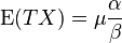
| Mean |
[1] 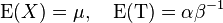 |
| Mode |
 |
| Variance |
[1] 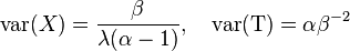 |
In probability theory and statistics, the normal-gamma distribution (or Gaussian-gamma distribution) is a bivariate four-parameter family of continuous probability distributions. It is the conjugate prior of a normal distribution with unknown mean and precision.[2]
Definition
For a pair of random variable, (X,T), suppose that the conditional distribution of X given T is given by
meaning that the conditional distribution is a normal distribution with mean  and precision
  — equivalently, with variance
Suppose also that the marginal distribution of T is given by
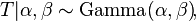
where this means that T has a gamma distribution. Here λ, α and β are parameters of the joint distribution.
Then (X,T) has a normal-gamma distribution, and this is denoted by

Properties
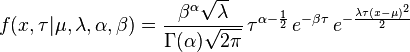
Probability density function
The joint probability density function of (X,T) is
Marginal distributions
By construction, the marginal distribution over  is a gamma distribution, and the conditional distribution over
  given is a Gaussian distribution. The marginal distribution over is a three-parameter non-standardized Student's t-distribution with parameters
 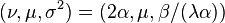 .
.
Exponential family
The normal-gamma distribution is a four-parameter exponential family with natural parameters  and natural statistics
 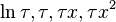 .
.
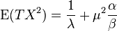
Moments of the natural statistics
The following moments can be easily computed using the moment generating function of the sufficient statistic:
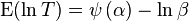 , where
  is the digamma function,
 ,
, ,
, .
.
Scaling
If  then for any b > 0, (bX,bT) is distributed as
Posterior distribution of the parameters
Assume that x is distributed according to a normal distribution with unknown mean and precision .

and that the prior distribution on and ,  , has a normal-gamma distribution

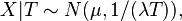
for which the density π satisfies
![\pi(\mu,\tau) \propto \tau^{\alpha_0-\frac{1}{2}}\,\exp[{-\beta_0\tau}]\,\exp[{ -\frac{\lambda_0\tau(\mu-\mu_0)^2}{2}}].](../I/m/7933b5ac52d06fda0290950be9229124.png)
Given a dataset  , consisting of
  independent and identically distributed random variables (i.i.d),
  , the posterior distribution of and given this dataset can be analytically determined by Bayes' theorem. Explicitly,
 ,
,
where  is the likelihood of the data given the parameters.
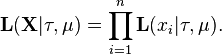
Since the data are i.i.d, the likelihood of the entire dataset is equal to the product of the likelihoods of the individual data samples:
This expression can be simplified as follows:
![\begin{align}
\mathbf{L}(\mathbf{X} | \tau, \mu) & \propto \prod_{i=1}^n \tau^{1/2} \exp[\frac{-\tau}{2}(x_i-\mu)^2] \\
& \propto \tau^{n/2} \exp[\frac{-\tau}{2}\sum_{i=1}^n(x_i-\mu)^2] \\
& \propto \tau^{n/2} \exp[\frac{-\tau}{2}\sum_{i=1}^n(x_i-\bar{x} +\bar{x} -\mu)^2] \\
& \propto \tau^{n/2} \exp[\frac{-\tau}{2}\sum_{i=1}^n\left((x_i-\bar{x})^2 + (\bar{x} -\mu)^2\right)] \\
& \propto \tau^{n/2} \exp[\frac{-\tau}{2}\left(n s + n(\bar{x} -\mu)^2\right)] ,
\end{align}](../I/m/d6ed806d33284ca09d08e493f2861132.png)
where  , the mean of the data samples, and
 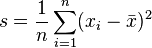 , the sample variance.
The posterior distribution of the parameters is proportional to the prior times the likelihood.
![\begin{align}
\mathbf{P}(\tau, \mu | \mathbf{X}) &\propto \mathbf{L}(\mathbf{X} | \tau,\mu) \pi(\tau,\mu) \\
&\propto \tau^{n/2} \exp[\frac{-\tau}{2}\left(n s + n(\bar{x} -\mu)^2\right)]
\tau^{\alpha_0-\frac{1}{2}}\,\exp[{-\beta_0\tau}]\,\exp[{ -\frac{\lambda_0\tau(\mu-\mu_0)^2}{2}}] \\
&\propto \tau^{\frac{n}{2} + \alpha_0 - \frac{1}{2}}\exp[-\tau \left( \frac{1}{2} n s + \beta_0 \right) ] \exp\left[- \frac{\tau}{2}\left(\lambda_0(\mu-\mu_0)^2 + n(\bar{x} -\mu)^2\right)\right] \\
\end{align}](../I/m/d9283b6b41b33cb5766dea5d1028e130.png)
The final exponential term is simplified by completing the square.
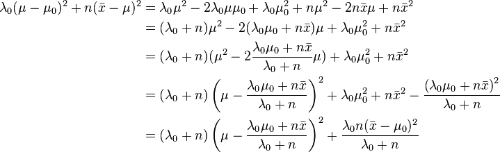
On inserting this back into the expression above,
![\begin{align}
\mathbf{P}(\tau, \mu | \mathbf{X}) & \propto \tau^{\frac{n}{2} + \alpha_0 - \frac{1}{2}} \exp \left[-\tau \left( \frac{1}{2} n s + \beta_0 \right) \right] \exp \left[- \frac{\tau}{2} \left( \left(\lambda_0 + n \right) \left(\mu- \frac{\lambda_0 \mu_0 + n \bar{x}}{\lambda_0 + n} \right)^2 + \frac{\lambda_0 n (\bar{x} - \mu_0 )^2}{\lambda_0 +n} \right) \right]\\
& \propto \tau^{\frac{n}{2} + \alpha_0 - \frac{1}{2}} \exp \left[-\tau \left( \frac{1}{2} n s + \beta_0 + \frac{\lambda_0 n (x - \mu_0 )^2}{2(\lambda_0 +n)} \right) \right] \exp \left[- \frac{\tau}{2} \left(\lambda_0 + n \right) \left(\mu- \frac{\lambda_0 \mu_0 + n \bar{x}}{\lambda_0 + n} \right)^2 \right]
\end{align}](../I/m/cf64db74f9d813e99e79f187f231c18b.png)
This final expression is in exactly the same form as a Normal-Gamma distribution, i.e.,

Interpretation of parameters
The interpretation of parameters in terms of pseudo-observations is as follows:
- The new mean takes a weighted average of the old pseudo-mean and the observed mean, weighted by the number of associated (pseudo-)observations.
- The precision was estimated from
 pseudo-observations (i.e. possibly a different number of pseudo-observations, to allow the variance of the mean and precision to be controlled separately) with sample mean and sample variance
  (i.e. with sum of squared deviations
  ).
). - The posterior updates the number of pseudo-observations (
 ) simply by adding up the corresponding number of new observations ().
 - The new sum of squared deviations is computed by adding the previous respective sums of squared deviations. However, a third "interaction term" is needed because the two sets of squared deviations were computed with respect to different means, and hence the sum of the two underestimates the actual total squared deviation.
As a consequence, if one has a prior mean of  from
from  samples and a prior precision of
  from
from  samples, the prior distribution over and is
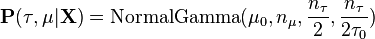
and after observing samples with mean and variance  , the posterior probability is

Note that in some programming languages, such as Matlab, the gamma distribution is implemented with the inverse definition of  , so the fourth argument of the Normal-Gamma distribution is
  .
.
Generating normal-gamma random variates
Generation of random variates is straightforward:
- Sample from a gamma distribution with parameters
 and
and - Sample from a normal distribution with mean and variance

Related distributions
- The normal-inverse-gamma distribution is essentially the same distribution parameterized by variance rather than precision
- The normal-exponential-gamma distribution
Notes
References
- Bernardo, J.M.; Smith, A.F.M. (1993) Bayesian Theory, Wiley. ISBN 0-471-49464-X
- Dearden et al. "Bayesian Q-learning", Proceedings of the Fifteenth National Conference on Artificial Intelligence (AAAI-98), July 26–30, 1998, Madison, Wisconsin, USA.