Non-negative least squares

Regression analysis
Models
Linear regression Simple regression Ordinary least squares Polynomial regression General linear model
Generalized linear model Discrete choice Logistic regression Multinomial logit Mixed logit Probit Multinomial probit Ordered logit Ordered probit Poisson
Multilevel model Fixed effects Random effects Mixed model
Nonlinear regression Nonparametric Semiparametric Robust Quantile Isotonic Principal components Least angle Local Segmented
Errors-in-variables
Estimation
Least squares Ordinary least squares Linear (math) Partial Total Generalized Weighted Non-linear Non-negative Iteratively reweighted Ridge regression LASSO
Least absolute deviations Bayesian Bayesian multivariate
Background
Regression model validation Mean and predicted response Errors and residuals Goodness of fit Studentized residual Gauss–Markov theorem
Statistics portal

In mathematical optimization, the problem of non-negative least squares (NNLS) is a constrained version of the least squares problem where the coefficients are not allowed to become negative. That is, given a matrix A and a (column) vector of response variables y, the goal is to find^[1]

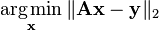subject to x ≥ 0.

Here, x ≥ 0 means that each component of the vector x should be non-negative and ‖·‖₂ denotes the Euclidean norm.

Non-negative least squares problems turn up as subproblems in matrix decomposition, e.g. in algorithms for PARAFAC^[2] and non-negative matrix/tensor factorization.^[3] The latter can be considered a generalization of NNLS.^[1]

Quadratic programming version

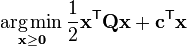
The NNLS problem is equivalent to a quadratic programming problem

,

where Q = AᵀA and c = −Aᵀ y. This problem is convex as Q is positive semidefinite and the non-negativity constraints form a convex feasible set.^[4]

Algorithms

The first widely used algorithm for solving this problem is an active set method published by Lawson and Hanson in their 1974 book Solving Least Squares Problems.^[5]:291 In pseudocode, this algorithm looks as follows:^[1][2]

# Inputs
A : matrix of shape (m, n)
y : vector of length m
tol : tolerance for the stopping criterion

# Initialization
P ← ∅
R ← {1, ..., n}
x ← zero-vector of length n
w ← Aᵀ(y − Ax)

while R ≠ ∅ and max(w) > tol
    j ← index of max(w) in w
    add j to P
    remove j from R
    # Aᴾ is A restricted to the variables included in P
    sᴾ ← ((Aᴾ)ᵀ Aᴾ)⁻¹ (Aᴾ)ᵀy
    while min(sᴾ) ≤ 0
        α ← min(xᵢ / (xᵢ - sᵢ) for i in P, sᵢ ≤ 0)
        x ← x + α(s - x)
        Move to R all indexes j in P such that xj = 0
        sᴾ ← ((Aᴾ)ᵀ Aᴾ)⁻¹ (Aᴾ)ᵀy
        sᴿ ← 0
    x ← s
    w ← Aᵀ(y − Ax)

This algorithm takes a finite number of steps to reach a solution and smoothly improves its candidate solution as it goes (so it can find good approximate solutions when cut off at a reasonable number of iterations), but is very slow in practice, owing largely to the computation of the pseudoinverse ((Aᴾ)ᵀ Aᴾ)⁻¹.^[1] Variants of this algorithm are available in Matlab as the routine lsqnonneg^[1] and in SciPy as optimize.nnls.^[6]

Many improved algorithms have been suggested since 1974.^[1] Fast NNLS (FNNLS) is an optimized version of the Lawson—Hanson algorithm.^[2] Other algorithms include variants of Landweber's gradient descent method^[7] and coordinate-wise optimization based on the quadratic programming problem above.^[4] Lawson and Hanson themselves have generalized it to handle general bounded-variable least squares (BLVS) problems, with upper and lower bounds αᵢ ≤ xᵢ ≤ βᵢ.^[5]:291

References

See also

• M-matrix
• Perron–Frobenius theorem

References

- ↑ 1.0 1.1 1.2 1.3 1.4 1.5 Chen, Donghui; Plemmons, Robert J. (2009). Nonnegativity constraints in numerical analysis. Symposium on the Birth of Numerical Analysis.
- ↑ 2.0 2.1 2.2 Bro, R.; De Jong, S. (1997). "A fast non-negativity-constrained least squares algorithm". Journal of Chemometrics 11 (5): 393. doi:10.1002/(SICI)1099-128X(199709/10)11:5<393::AID-CEM483>3.0.CO;2-L.
- ↑ Lin, Chih-Jen (2007). "Projected Gradient Methods for Nonnegative Matrix Factorization". Neural Computation 19 (10): 2756–2779. doi:10.1162/neco.2007.19.10.2756. PMID 17716011.
- ↑ 4.0 4.1 Franc, V. C.; Hlaváč, V. C.; Navara, M. (2005). "Sequential Coordinate-Wise Algorithm for the Non-negative Least Squares Problem". Computer Analysis of Images and Patterns. Lecture Notes in Computer Science 3691. p. 407. doi:10.1007/11556121_50. ISBN 978-3-540-28969-2.
- ↑ 5.0 5.1 Lawson, Charles L.; Hanson, Richard J. (1995). Solving Least Squares Problems. SIAM.
- ↑ "scipy.optimize.nnls". SciPy v0.13.0 Reference Guide. Retrieved 25 January 2014.
- ↑ Johansson, B. R.; Elfving, T.; Kozlov, V.; Censor, Y.; Forssén, P. E.; Granlund, G. S. (2006). "The application of an oblique-projected Landweber method to a model of supervised learning". Mathematical and Computer Modelling 43 (7–8): 892. doi:10.1016/j.mcm.2005.12.010.