Newsvendor model

The newsvendor (or newsboy or single-period^[1] or perishable ^[2]) model is a mathematical model in operations management and applied economics used to determine optimal inventory levels. It is (typically) characterized by fixed prices and uncertain demand for a perishable product. If the inventory level is $q$ , each unit of demand above $q$ is lost in potential sales. This model is also known as the Newsvendor Problem or Newsboy Problem by analogy with the situation faced by a newspaper vendor who must decide how many copies of the day's paper to stock in the face of uncertain demand and knowing that unsold copies will be worthless at the end of the day.

History

The mathematical problem appears to date from 1888^[3] where Edgeworth used the central limit theorem to determine the optimal cash reserves to satisfy random withdrawals from depositors.^[4] The modern formulation dates from a 1951 paper in Econometrica by Kenneth Arrow, T. Harris, and Jacob Marshak.^[5]

Profit function

The standard newsvendor profit function is

\pi =E\left[p\min (q,D)\right]-cq

where $D$ is a random variable with probability distribution $F$ representing demand, each unit is sold for price $p$ and purchased for price $c$ , $q$ is the number of units stocked, and $E$ is the expectation operator. The solution to the optimal stocking quantity of the newsvendor which maximizes expected profit is:

Critical fractile formula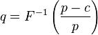

$q=F^{-1}\left( \frac{p-c}{p}\right)$

where $F^{-1}$ denotes the inverse cumulative distribution function of $D$ .

Intuitively, this ratio, referred to as the critical fractile, balances the cost of being understocked (a lost sale worth $(p-c)$ ) and the total costs of being either overstocked or understocked (where the cost of being overstocked is the inventory cost, or $c$ so total cost is simply $p$ ).

The critical fractile formula is known as Littlewood's rule in the yield management literature.

Numerical Examples

Uniform Distribution

Assume that: retail price is $p=7$ [$/unit] and purchase price is $c=5$ [$/unit]. Furthermore the $D$ demand follows a uniform distribution (continuous) between $D_\min = 50$ and $D_\max = 80$ .

q_\text{opt}=F^{-1}\left( \frac{7-5}{7}\right)=F^{-1}\left( 0.285 \right) = D_\min+(D_\max-D_\min) \cdot 0.285 = 58.55\approx59.

Therefore optimal inventory level is approximately 59 units.

Normal Distribution

Assume that: retail price is $p=7$ [$/unit] and purchase price is $c=5$ [$/unit]. Furthermore the $D$ demand follows a normal distribution with a mean, $\mu$ , demand of 50 and a standard deviation, $\sigma$ , of 20.

q_\text{opt}=F^{-1}\left( \frac{7-5}{7}\right)=\mu + \sigma Z^{-1}\left( 0.285 \right) = 50 + 20 \cdot -0.56595 = 38.68\approx 39.

Therefore optimal inventory level is approximately 39 units.

q opt = Mu + sigma x zinv x (2/7) Go to MSExcel. NORMSINV (0.285714) = - 0.56595 Therefore q= 50 + 20 (-0.56595) = 38.69 units

Lognormal Distribution

Assume that: retail price is $p=7$ [$/unit] and purchase price is $c=5$ [$/unit]. Furthermore the $D$ demand follows a lognormal distribution with a mean demand of 50, $\mu$ , and a standard deviation, $\sigma$ , of 0.2.

q_\text{opt}=F^{-1}\left(\frac{7-5}{7}\right)=\mu e^{Z^{-1}\left(0.285\right) \sigma} = 50 e^{\left(0.2 \cdot -0.56595 \right)} = 44.64\approx 45.

Therefore optimal inventory level is approximately 45 units.

Extreme situation

If $p<c$ (i.e. the retail price is less than the purchase price), the numerator becomes negative. In this situation, it isn't worth keeping any item in the inventory.

Cost based optimization of inventory level

Assuming that the 'newsvendor' is in fact a small company who wants to produce goods to an uncertain market. In this more general situation the cost function of the newsvendor (company) can be formulated in the following manner:

K(q) = c_f + c_v (q-x) + p E\left[\max(D-q,0)\right] + h E\left[\max(q-D,0)\right]

where the individual parameters are the following:

$c_f$ – fixed cost. This cost always exists when the production of a series is started. [$/production]
$c_v$ – variable cost. This cost type expresses the production cost of one product. [$/product]
$q$ – The product quantity in the inventory. The decision of the inventory control policy concerns the product quantity in the inventory after the product decision. This parameter includes the initial inventory as well. If nothing is produced, then this quantity is equal to the initial quantity, i.e. concerning the existing inventory.
$x$ – Initial inventory level. We assume that the supplier possesses $x$ products in the inventory at the beginning of the demand of the delivery period.
$p$ – penalty cost (or back order cost). If there is less raw material in the inventory than needed to satisfy the demands, this is the penalty cost of the unsatisfied orders. [$/product]
$E[D]$ – Expected value of the $D$ stochastic variable.
$D$ – This means the demand from the receiver for the product, which is an optional probability variable. [unit]
$h$ – inventory and stock holding cost. [$ / product]

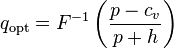
On the basis of the cost function the determination of the optimal inventory level is a minimization problem. So in the long run the amount of cost-optimal end-product can be calculated on the basis of the following relation:^[1]

q_\text{opt} = F^{-1}\left( \frac{p-c_v}{p+h}\right)

References

↑ 1.0 1.1 William J. Stevenson, Operations Management. 10th edition, 2009; page 581
↑ Malakooti, Behnam (2013). Operations and Production Systems with Multiple Objectives. John Wiley & Sons. ISBN 978-1-118-58537-5.
↑ F. Y. Edgeworth (1888). "The Mathematical Theory of Banking". Journal of the Royal Statistical Society 51 (1): 113–127. JSTOR 2979084.
↑ Guillermo Gallego (18 Jan 2005). "IEOR 4000 Production Management Lecture 7" (PDF). Columbia University. Retrieved 30 May 2012.
↑ K.J. Arrow, T. Harris, Jacob Marshak, Optimal Inventory Policy, Econometrica 1951