Nakagami distribution
|
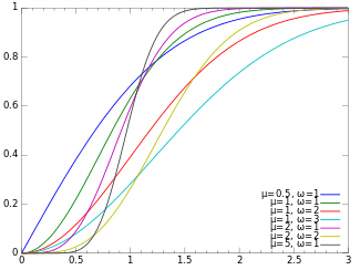
Probability density function
| |
|
Cumulative distribution function
| |
| Parameters |
 shape (real) shape (real) spread (real) spread (real) |
|---|---|
| Support |
 |
 | |
| CDF |
 |
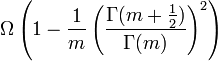
| Mean |
 |
| Median |
 |
| Mode |
 |
| Variance |
 |

The Nakagami distribution or the Nakagami-m distribution is a probability distribution related to the gamma distribution. It has two parameters: a shape parameter  and a second parameter controlling spread,
  .
.
Characterization
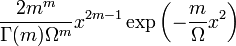
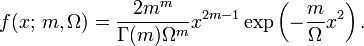
Its probability density function (pdf) is[1]
Its cumulative distribution function is[1]
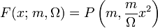
where P is the incomplete gamma function (regularized).

Parameter estimation
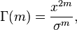
The parameters and are[2]
![m = \frac{\operatorname{E}^2 \left[X^2 \right]}
{\operatorname{Var} \left[X^2 \right]},](../I/m/4ccade4fe14336166cd60dbd71e50535.png)
and
![\Omega = \operatorname{E} \left[X^2 \right].](../I/m/3a0aca9577669b34c220da0dafa5834a.png)
An alternative way of fitting the distribution is to re-parametrize and m as σ = Ω/m and m.[3] Then, by taking the derivative of log likelihood with respect to each of the new parameters, the following equations are obtained and these can be solved using the Newton-Raphson method:
and

It is reported by authors that modelling data with Nakagami distribution and estimating parameters by above mention method results in better performance for low data regime compared to moments based methods.
Generation
The Nakagami distribution is related to the gamma distribution.
In particular, given a random variable  , it is possible to obtain a random variable
  , by setting
  ,
,  , and taking the square root of
  :
:
 .
.
The Nakagami distribution  can be generated from the chi distribution with parameter
  set to
  and then following it by a scaling transformation of random variables. That is, a Nakagami random variable
  is generated by a simple scaling transformation on a Chi-distributed random variable
  as below:
History and applications
The Nakagami distribution is relatively new, being first proposed in 1960.[4] It has been used to model attenuation of wireless signals traversing multiple paths.[5]
References
- ↑ 1.0 1.1 Laurenson, Dave (1994). "Nakagami Distribution". Indoor Radio Channel Propagation Modelling by Ray Tracing Techniques. Retrieved 2007-08-04.
- ↑ R. Kolar, R. Jirik, J. Jan (2004) "Estimator Comparison of the Nakagami-m Parameter and Its Application in Echocardiography", Radioengineering, 13 (1), 8–12
- ↑ Mitra, Rangeet; Mishra, Amit Kumar; Choubisa, Tarun (2012). "Maximum Likelihood Estimate of Parameters of Nakagami-m Distribution". International Conference on Communications, Devices and Intelligent Systems (CODIS), 2012: 9-12.
- ↑ Nakagami, M. (1960) "The m-Distribution, a general formula of intensity of rapid fading". In William C. Hoffman, editor, Statistical Methods in Radio Wave Propagation: Proceedings of a Symposium held June 18-20, 1958, pp 3-36. Pergamon Press.
- ↑ Parsons, J. D. (1992) The Mobile Radio Propagation Channel. New York: Wiley.