Moran process

A Moran process or Moran model is a simple stochastic process used in biology to describe finite populations. The process is named after Patrick Moran, who first proposed the model in 1958.^[1] It can be used to model variety-increasing processes such as mutation as well as variety-reducing effects such as genetic drift and natural selection. The process can describe the probabilistic dynamics in a finite population of constant size N in which two alleles A and B are competing for dominance. The two alleles are considered to be true replicators (i.e. entities that make copies of themselves).

In each time step a random individual (which is of either type A or B) is chosen for reproduction and a random individual is chosen for death; thus ensuring that the population size remains constant. To model selection, one type has to have a higher fitness and is thus more likely to be chosen for reproduction. The same individual can be chosen for death and for reproduction in the same step.

Neutral drift

Neutral drift is the idea that a neutral mutation can spread throughout a population, so that eventually the original allele is lost. A neutral mutation does not bring any fitness advantage or disadvantage to its bearer. The simple case of the Moran process can describe this phenomenon.

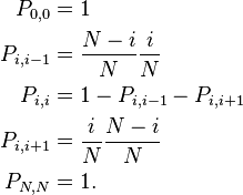
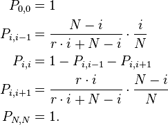
If the number of A individuals is given by i then the Moran process is defined on the state space $i = 0, ..., N$ . Since the number of A individuals can change at most by one at each time step, a transition exists only between state i and state $i - 1, i$ and $i + 1$ . Thus the transition matrix of the stochastic process is tri-diagonal in shape and the transition probabilities are

\begin{align} P_{0,0}&=1\\ P_{i,i-1} &= \frac{N-i}{N} \frac{i}{N}\\ P_{i,i} &= 1- P_{i,i-1} - P_{i,i+1}\\ P_{i,i+1} &= \frac{i}{N} \frac{N-i}{N}\\ P_{N,N}&=1. \end{align}

The entry $P_{i,j}$ denotes the probability to go from state i to state j. To understand the formulas for the transition probabilities one has to look at the definition of the process which states that always one individual will be chosen for reproduction and one is chosen for death. Once the A individuals have died out, they will never be reintroduced into the population since the process does not model mutations (A cannot be reintroduced into the population once it has died out and vice versa) and thus $P_{0,0}=1$ . For the same reason the population of A individuals will always stay N once they have reached that number and taken over the population and thus $P_{N,N}=1$ . The states 0 and N are called absorbing while the states $1, ..., N - 1$ are called transient. The intermediate transition probabilities can be explained by considering the first term to be the probability to choose the individual whose abundance will increase by one and the second term the probability to choose the other type for death. Obviously, if the same type is chosen for reproduction and for death, then the abundance of one type does not change.

Eventually the population will reach one of the absorbing states and then stay there forever. In the transient states, random fluctuations will occur but eventually the population of A will either go extinct or reach fixation. This is one of the most important differences to deterministic processes which cannot model random events. The expected value and the variance of the number of A individuals $X (t)$ at timepoint t can be computed when an initial state $X (0) = i$ is given:

\begin{align} E[X(t)|X(0) = i] &= i \\ Var(X(t)|X(0) = i) &= \tfrac{2i}{N} \left(1-\tfrac{i}{N} \right ) \frac{1- \left(1-\frac{2}{N^2} \right )^t}{\frac{2}{N^2}} \end{align}

For a mathematical derivation of the equation above, click on "show" to reveal

For the expected value the calculation runs as follows. Writing $p = i / N,$

\begin{align} E [X(t) | X(t-1) = i] &= (i-1)P_{i,i-1} + iP_{i,i} + (i+1)P_{i,i+1}\\ &= 2ip(1-p) + i(p^2 + (1-p)^2) \\ &= i. \end{align}

Writing $Y = X(t)$ and $Z = X(t-1)$ , and applying the law of total expectation, $E[Y] = E[E[Y|Z]] = E[Z].$ Applying the argument repeatedly gives $E[X(t)] = E[X(0)],$ or $E[X(t)|X(0) = i] = i.$

For the variance the calculation runs as follows. Writing $V_t = Var(X(t)|X(0) = i),$ we have

\begin{align} V_1 &= E \left[X(1)^2|X(0) = i \right] - E[X(1)|X(0)=i]^2 \\ &= (i-1)^2p(1-p) + i^2 \left (p^2+(1-p)^2 \right ) + (i+1)^2p(1-p) - i^2 \\ &= 2p(1-p) \end{align}

For all $t$ , $(X(t)|X(t-1) = i)$ and $(X(1)|X(0) = i)$ are identically distributed, so their variances are equal. Writing as before $Y = X(t)$ and $Z = X(t-1)$ , and applying the law of total variance,

\begin{align} Var(Y) &= E[Var(Y|Z)] + Var(E[Y|Z]) \\ &= E \left [\left (\frac{2Z}{N} \right) \left(1-\frac{Z}{N} \right ) \right ] + Var(Z)\\ &= \left(\frac{2E[Z]}{N} \right ) \left (1-\frac{E[Z]}{N} \right) + \left(1-\frac{2}{N^2}\right)Var(Z). \end{align}

If $X(0) = i$ , we obtain

V_t = V_1 + \left (1-\frac{2}{N^2} \right)V_{t-1}.

Rewriting this equation as

V_t - \frac{V_1}{\frac{2}{N^2}} = \left (1-\frac{2}{N^2} \right )\left(V_{t-1}-\frac{V_1}{\frac{2}{N^2}}\right) = \left (1-\frac{2}{N^2} \right)^{t-1} \left(V_1-\frac{V_1}{\frac{2}{N^2}}\right)

yields

V_t = V_1 \frac{1-\left (1-\frac{2}{N^2} \right)^t}{\frac{2}{N^2}}

as desired.

The probability of A to reach fixation is called fixation probability. For the simple Moran process this probability is $x i = i / N .$

Since all individuals have the same fitness, they also have the same chance of becoming the ancestor of the whole population; this probability is $1 / N$ and thus the sum of all i probabilities (for all A individuals) is just $i / N .$ The mean time to absorption starting in state i is given by

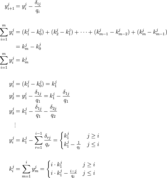
k_i = N \left[ \sum_{j=1}^{i} \frac{N-i}{N-j} + \sum_{j=i+1}^{N-1} \frac{i}{j} \right]

For a mathematical derivation of the equation above, click on "show" to reveal

The mean time spent in state j when starting in state i which is given by

k_i^j = \delta_{ij}+P_{i,i-1}k_{i-1}^j + P_{i,i}k_{i}^j + P_{i,i+1}k_{i+1}^j

Here $δ ij$ denotes the Kroenecker delta. This recursive equation can be solved using a new variable $q i$ so that $P_{i,i-1} = P_{i,i+1} = q_i$ and thus $P_{i,i} = 1-2 q_i$ and rewritten

k_{i+1}^j = 2 k_{i}^j- k_{i-1}^j -\frac{\delta_{ij}}{q_i}

The variable $y_i^{j} = k_{i}^j- k_{i-1}^j$ is used and the equation becomes

\begin{align} y_{i+1}^{j} &= y_i^{j} -\frac{\delta_{ij}}{q_i} \\ \\ \sum_{i=1}^m y_i^{j} &= (k_{1}^j- k_{0}^j) + (k_{2}^j- k_{1}^j) + \cdots + (k_{m-1}^j- k_{m-2}^j) + (k_{m}^j- k_{m-1}^j) \\ &= k_{m}^j - k_{0}^j \\ \sum_{i=1}^m y_i^{j} &= k_{m}^j \\ \\ y_1^{j} &= (k_{1}^j- k_{0}^j) = k_{1}^j \\ y_2^{j} &= y_1^{j} -\frac{\delta_{1j}}{q_1} = k_1^{j} -\frac{\delta_{1j}}{ q_1 } \\ y_3^{j} &= k_1^{j} -\frac{\delta_{1j}}{q_1} -\frac{\delta_{2j}}{ q_2 } \\ & \vdots \\ y_i^{j} &= k_1^{j} -\sum_{r=1}^{i-1} \frac{\delta_{rj}}{q_r} = \begin{cases} k_1^j & j \geq i\\ k_1^j - \frac{1}{q_j} & j \leq i \end{cases} \\ \\ k_i^j &= \sum_{m=1}^i y_m^{j} = \begin{cases} i \cdot k_1^j & j \geq i\\ i \cdot k_1^j - \frac{i-j}{q_j} & j \leq i \end{cases} \end{align}

Knowing that $k_N^j = 0$ and

q_j = P_{j,j+1}=\frac{j}{N} \frac{N-j}{N}

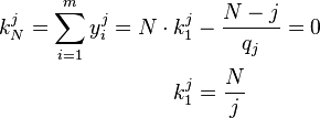
we can calculate $k_1^j$ :

\begin{align} k_N^j = \sum_{i=1}^m y_i^{j} = N \cdot k_1^j &- \frac{N-j}{q_j} = 0 \\ k_1^j &= \frac{N}{j} \end{align}

Therefore

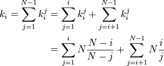
k_i^j = \begin{cases} \frac{i}{j} \cdot k_j^j & j \geq i\\ \frac{N - i}{N-j} \cdot k_j^j & j \leq i\end{cases}

with $k_j^j = N$ . Now $k i$ , the total time until fixation starting from state i, can be calculated

\begin{align} k_i = \sum_{j=1}^{N-1}k_i^j &= \sum_{j=1}^{i}k_i^j + \sum_{j=i+1}^{N-1}k_i^j \\ &= \sum_{j=1}^{i}N \frac{N-i}{N-j} + \sum_{j=i+1}^{N-1}N \frac{i}{j} \end{align}

For large N the approximation

\lim_{N\to \infty} k_i \approx -N^2 \left[ (1-x_i) \ln(1-x_i) + x_i \ln(x_i) \right]

holds.

Selection

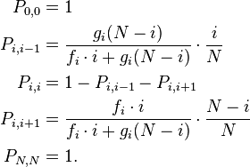
If one allele has a fitness advantage over the other allele, it will be more likely to be chosen for reproduction. This can be incorporated into the model if individuals with allele A have fitness $f_i$ and individuals with allele B have fitness $g i$ where i is the number of individuals of type A; thus describing a general birth-death process. The transition matrix of the stochastic process is tri-diagonal in shape and the transition probabilities are

\begin{align} P_{0,0}&=1 \\ P_{i,i-1} &= \frac{g_i (N-i) }{f_i \cdot i + g_i (N-i)} \cdot \frac{i}{N}\\ P_{i,i} &= 1- P_{i,i-1} - P_{i,i+1}\\ P_{i,i+1} &= \frac{f_i \cdot i}{f_i \cdot i + g_i (N-i)} \cdot \frac{N-i}{N}\\ P_{N,N}&=1. \end{align}

The entry $P_{i,j}$ denotes the probability to go from state i to state j. To understand the formulas for the transition probabilities one has to look again at the definition of the process and see that the fitness enters only the first term in the equations which is concerned with reproduction. Thus the probability that individual A is chosen for reproduction is not i / N any more but dependent on the fitness of A and thus

\frac{f_i \cdot i}{f_i \cdot i + g_i (N-i)}.

Also in this case, fixation probabilities when starting in state i is defined by recurrence

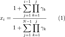
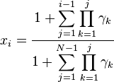
x_i = \begin{cases} 0 & i=0\\ \beta_i x_{i-1}+(1-\alpha_i-\beta_i)x_i+\alpha_ix_{i+1} & 1 \leq i \leq N-1\\ 1 & i =N \end{cases}

And the closed form is given by

x_i = \frac{{\displaystyle 1 + \sum_{j=1}^{i-1}\prod_{k=1}^{j}\gamma_k}} {{\displaystyle 1 + \sum_{j=1}^{N-1}\prod_{k=1}^{j}\gamma_k}} \qquad \text{(1)}

where $\gamma_i = P_{i,i-1} / P_{i,i+1}$ per definition and will just be $g_i / f_i$ for the general case.

For a mathematical derivation of the equation above, click on "show" to reveal

Also in this case, fixation probabilities can be computed, but the transition probabilities are not symmetric. The notation $P_{i,i+1}=\alpha_i, P_{i,i-1}=\beta_i, P_{i,i}=1-\alpha_i- \beta_i$ and $\gamma_i = \beta_i / \alpha_i$ is used. The fixation probability can be defined recursively and a new variable $y_i = x_i - x_{i-1}$ is introduced.

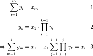
\begin{align} x_i &= \beta_i x_{i-1} + (1-\alpha_i - \beta_i)x_i + \alpha_i x_{i+1} \\ \beta_i (x_i - x_{i-1} ) &= \alpha_i (x_{i+1} - x_i ) \\ \gamma_i \cdot y_i &= y_{i+1} \end{align}

Now two properties from the definition of the variable $y i$ can be used to find a closed form solution for the fixation probabilities:

\begin{align} \sum_{i=1}^{m} y_i &= x_m && 1\\ y_k &= x_1 \cdot \prod_{l=1}^{k-1}\gamma_l && 2\\ \Rightarrow \sum_{m=1}^{i}y_m &= x_1 + x_1 \sum_{j=1}^{i-1}\prod_{k=1}^{j}\gamma_k = x_i && 3 \end{align}

Combining (3) and $x N = 1$ :

x_1 \left(1 + \sum_{j=1}^{N-1}\prod_{k=1}^{j}\gamma_k \right) = x_N = 1.

which implies:

x_1 = \frac{1}{1 + \sum_{j=1}^{N-1} \prod_{k=1}^{j}\gamma_k}

This in turn gives us:

x_i = \frac{{\displaystyle 1 + \sum_{j=1}^{i-1}\prod_{k=1}^{j}\gamma_k}}{{\displaystyle 1 + \sum_{j=1}^{N-1}\prod_{k=1}^{j}\gamma_k}}

This general case where the fitness of A and B depends on the abundance of each type is studied in evolutionary game theory.

Less complex results are obtained if a constant fitness difference r is assumed. Individuals of type A reproduce with a constant rate r and individuals with allele B reproduce with rate 1. Thus if A has a fitness advantage over B, r will be larger than one, otherwise it will be smaller than one. Thus the transition matrix of the stochastic process is tri-diagonal in shape and the transition probabilities are

\begin{align} P_{0,0}&=1\\ P_{i,i-1} &= \frac{N-i}{r \cdot i + N-i} \cdot \frac{i}{N}\\ P_{i,i} &= 1- P_{i,i-1} - P_{i,i+1}\\ P_{i,i+1} &= \frac{r \cdot i}{r \cdot i + N-i} \cdot \frac{N-i}{N}\\ P_{N,N}&=1. \end{align}

In this case $\gamma_i = 1/r$ is a constant factor for each composition of the population and thus the fixation probability from equation (1) simplifies to

x_i = \frac{1-r^{-i}} { 1-r^{-N} } \quad \Rightarrow \quad x_1 = \rho = \frac{1-r^{-1}} {1-r^{-N}} \qquad \text{(2)}

where the fixation probability of a single mutant A in a population of otherwise all B is often of interest and is denoted by $ρ$ .

Also in the case of selection, the expected value and the variance of the number of A individuals may be computed

\begin{align} E [ X(t) | X(t-1) = i ] &= p s \dfrac{1-p}{p s + 1} + i \\ Var( X(t+1) | X(t)=i) &=p(1-p)\dfrac{ (s+1) + (p s + 1)^2 }{(p s +1)^2} \end{align}

where $p = i / N,$ and $r = 1 + s$ .

For a mathematical derivation of the equation above, click on "show" to reveal

For the expected value the calculation runs as follows

\begin{align} E [ \Delta(1) | X(0) = i ] &= (i-1-i) \cdot P_{i,i-1} + (i-i) \cdot P_{i,i} + (i+1-i) \cdot P_{i,i+1} \\ &= -\frac{N-i}{r i + N -i} \frac{i}{N} + \frac{ri}{r i + N -i} \frac{N-i}{N} \\ &= -\frac{(N-i)i}{(r i + N -i)N} + \frac{i(N-i)}{(r i + N -i)N} + \frac{si(N-i)}{(r i + N -i)N} \\ &= p s \dfrac{1-p}{p s + 1}\\ E [ X(t) | X(t-1) = i ] &= p s \dfrac{1-p}{p s + 1}+i \end{align}

For the variance the calculation runs as follows, using the variance of a single step

\begin{align} Var( X(t+1) | X(t)=i) &= Var(X(t)) + Var(\Delta(t+1)| X(t)=i) \\ &= 0 + E\left [\Delta(t+1)^2| X(t)=i \right ] - E[\Delta(t+1)| X(t)=i]^2\\ &= (i-1-i)^2 \cdot P_{i,i-1} + (i-i)^2 \cdot P_{i,i} + (i+1-i)^2 \cdot P_{i,i+1} - E[\Delta(t+1)| X(t)=i]^2\\ &= P_{i,i-1} + P_{i,i+1} - E[\Delta(t+1)| X(t)=i]^2\\ &= \frac{(N-i)i}{(r i + N -i)N} + \frac{(N-i)i(1+s)}{(r i + N -i)N} - E[\Delta(t+1)| X(t)=i]^2\\ &= i (N-i)\frac{2+s}{(r i + N -i)N} - E[\Delta(t+1)| X(t)=i]^2\\ &= i (N-i)\frac{2+s}{(r i + N -i)N} - \left (p s \dfrac{1-p}{ps + 1} \right )^2\\ &= p(1-p)\frac{2+s (ps + 1)}{(ps + 1)^2} - p(1-p) \frac{p s^2(1-p)}{(p s + 1)^2}\\ &= p(1-p)\dfrac{2+2ps + s + p^2 s^2}{(ps +1)^2} \end{align}

Rate of evolution

In a population of all B individuals, a single mutant A will take over the whole population with the probability

\rho = \frac{1-r^{-1}}{1-r^{-N}}. \qquad \text{(2)}

If the mutation rate (to go from the B to the A allele) in the population is u then the rate with which one member of the population will mutate to A is given by $N \times u$ and the rate with which the whole population goes from all B to all A is the rate that a single mutant A arises times the probability that it will take over the population (fixation probability):

R = N \cdot u \cdot \rho = u \quad \text{if} \quad \rho = \frac{1}{N}.

Thus if the mutation is neutral (i.e. the fixation probability is just 1/N) then the rate with which an allele arises and takes over a population is independent of the population size and is equal to the mutation rate. This important result is the basis of the neutral theory of evolution and suggests that the number of observed point mutations in the genomes of two different species would simply be given by the mutation rate multiplied by two times the time since divergence. Thus the neutral theory of evolution provides a molecular clock, given that the assumptions are fulfilled which may not be the case in reality.

References

↑ Moran, P. A. P. (1958). "Random processes in genetics". Mathematical Proceedings of the Cambridge Philosophical Society 54 (1): 60–71. doi:10.1017/S0305004100033193.

External links

"Evolutionary Dynamics on Graphs".

Stochastic processes

Discrete time	Bernoulli process Branching process Chinese restaurant process Galton–Watson process Independent and identically distributed random variables Markov chain Moran process Random walk Loop-erased Self-avoiding

Continuous time	Bessel process Birth–death process Brownian motion Bridge Excursion Fractional Geometric Meander Cauchy process Contact process Continuous-time random walk Cox process Diffusion process Empirical process Feller process Fleming–Viot process Gamma process Hunt process Interacting particle systems Itō diffusion Itō process Jump diffusion Jump process Lévy process Local time Markov additive process McKean–Vlasov process Ornstein–Uhlenbeck process Poisson process Compound Non-homogeneous Point process Schramm–Loewner evolution Semimartingale Sigma-martingale Stable process Superprocess Telegraph process Variance gamma process Wiener process Wiener sausage

Both	Branching process Gaussian process Hidden Markov model (HMM) Markov process Martingale Differences Local Sub- Super- Random dynamical system Regenerative process Renewal process White noise

Fields and other	Dirichlet process Gaussian random field Gibbs measure Hopfield model Ising model Potts model Boolean network Markov random field Percolation Pitman–Yor process Point process Cox Poisson Random field Random graph

Time series models	Autoregressive conditional heteroskedasticity (ARCH) model Autoregressive integrated moving average (ARIMA) model Autoregressive (AR) model Autoregressive–moving-average (ARMA) model Generalized autoregressive conditional heteroskedasticity (GARCH) model Moving-average (MA) model

Financial models	Black–Derman–Toy Black–Karasinski Black–Scholes Chen Constant elasticity of variance (CEV) Cox–Ingersoll–Ross (CIR) Garman–Kohlhagen Heath–Jarrow–Morton (HJM) Heston Ho–Lee Hull–White LIBOR market SABR volatility Vašíček

Actuarial models	Bühlmann Cramér–Lundberg Risk process Sparre–Anderson

Queueing models	Bulk Fluid Generalized queueing network M/G/1 M/M/1 M/M/c

Properties	Càdlàg paths Continuous Continuous paths Ergodic Exchangeable Feller-continuous Gauss–Markov Markov Mixing Piecewise deterministic Predictable Progressively measurable Self-similar Stationary Time-reversible

Limit theorems	Central limit theorem Donsker's theorem Doob's martingale convergence theorems Ergodic theorem Fisher–Tippett–Gnedenko theorem Large deviation principle Law of large numbers (weak/strong) Law of the iterated logarithm Maximal ergodic theorem Sanov's theorem

Inequalities	Burkholder–Davis–Gundy Doob's martingale Kunita–Watanabe

Tools	Cameron–Martin formula Convergence of random variables Doléans-Dade exponential Doob decomposition theorem Doob–Meyer decomposition theorem Doob's optional stopping theorem Dynkin's formula Feynman–Kac formula Filtration Girsanov theorem Infinitesimal generator Itō integral Itō's lemma Kolmogorov continuity theorem Kolmogorov extension theorem Lévy–Prokhorov metric Malliavin calculus Martingale representation theorem Optional stopping theorem Prohorov theorem Quadratic variation Reflection principle Skorokhod integral Skorokhod's representation theorem Skorokhod space Snell envelope Stochastic differential equation Tanaka Stopping time Stratonovich integral Uniform integrability Usual hypotheses Wiener space Classical Abstract

Disciplines	Actuarial mathematics Econometrics Ergodic theory Extreme value theory (EVT) Large deviations theory Mathematical finance Mathematical statistics Probability theory Queueing theory Renewal theory Ruin theory Statistics Stochastic analysis Time series analysis Machine learning

List of topics Category

Moran process

Neutral drift

Selection

Rate of evolution

References

Further reading

External links