Mooney–Rivlin solid
| Continuum mechanics | ||||
|---|---|---|---|---|
 | ||||
|
Laws
|
||||
In continuum mechanics, a Mooney–Rivlin solid[1][2] is a hyperelastic material model where the strain energy density function  is a linear combination of two invariants of the left Cauchy–Green deformation tensor
  . The model was proposed by Melvin Mooney in 1940 and expressed in terms of invariants by Ronald Rivlin in 1948.
The strain energy density function for an incompressible Mooney–Rivlin material is[3][4]

where  and
and  are empirically determined material constants, and
  and
and  are the first and the second invariant of the unimodular component of the left Cauchy–Green deformation tensor:[5]
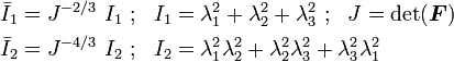
where  is the deformation gradient. For an incompressible material,
  .
.
Derivation
The Mooney–Rivlin model is a special case of the generalized Rivlin model (also called polynomial hyperelastic model[6]) which has the form
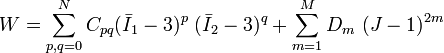
with  where
where  are material constants related to the distortional response and
  are material constants related to the volumetric response. For a compressible Mooney–Rivlin material
  and we have

If  we obtain a neo-Hookean solid, a special case of a Mooney–Rivlin solid.
For consistency with linear elasticity in the limit of small strains, it is necessary that

where  is the bulk modulus and
  is the shear modulus.
Cauchy stress in terms of strain invariants and deformation tensors
The Cauchy stress in a compressible hyperelastic material with a stress free reference configuration is given by
![\boldsymbol{\sigma} = \cfrac{2}{J}\left[\cfrac{1}{J^{2/3}}\left(\cfrac{\partial{W}}{\partial \bar{I}_1} + \bar{I}_1~\cfrac{\partial{W}}{\partial \bar{I}_2}\right)\boldsymbol{B} -
\cfrac{1}{J^{4/3}}~\cfrac{\partial{W}}{\partial \bar{I}_2}~\boldsymbol{B} \cdot\boldsymbol{B} \right] + \left[\cfrac{\partial{W}}{\partial J} -
\cfrac{2}{3J}\left(\bar{I}_1~\cfrac{\partial{W}}{\partial \bar{I}_1} + 2~\bar{I}_2~\cfrac{\partial{W}}{\partial \bar{I}_2}\right)\right]~\boldsymbol{\mathit{1}}](../I/m/74b172f8e241a41aa805133430a6105a.png)
For a compressible Mooney–Rivlin material,
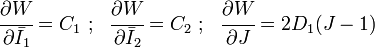
Therefore, the Cauchy stress in a compressible Mooney–Rivlin material is given by
![\boldsymbol{\sigma} = \cfrac{2}{J}\left[\cfrac{1}{J^{2/3}}\left(C_1 + \bar{I}_1~C_2\right)\boldsymbol{B} -
\cfrac{1}{J^{4/3}}~C_2~\boldsymbol{B} \cdot\boldsymbol{B} \right] + \left[2D_1(J-1)-
\cfrac{2}{3J}\left(C_1\bar{I}_1 + 2C_2\bar{I}_2~\right)\right]\boldsymbol{\mathit{1}}](../I/m/d04c0aa5c4eee115f9a533cec1046d6c.png)
It can be shown, after some algebra, that the pressure is given by
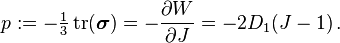
The stress can then be expressed in the form
![\boldsymbol{\sigma} = \cfrac{1}{J}\left[-p~\boldsymbol{\mathit{1}} + \cfrac{2}{J^{2/3}}\left(C_1 + \bar{I}_1~C_2\right)\boldsymbol{B} -
\cfrac{2}{J^{4/3}}~C_2~\boldsymbol{B}\cdot\boldsymbol{B} -\cfrac{2}{3}\left(C_1\,\bar{I}_1 + 2C_2\,\bar{I}_2\right)\boldsymbol{\mathit{1}}\right] \,.](../I/m/10f833e634f2428c23d82a4602252b76.png)
The above equation is often written as
![\boldsymbol{\sigma} = \cfrac{1}{J}\left[-p~\boldsymbol{\mathit{1}} + 2\left(C_1 + \bar{I}_1~C_2\right)\bar{\boldsymbol{B}} -
2~C_2~\bar{\boldsymbol{B}}\cdot\bar{\boldsymbol{B}} -\cfrac{2}{3}\left(C_1\,\bar{I}_1 + 2C_2\,\bar{I}_2\right)\boldsymbol{\mathit{1}}\right] \quad \text{where} \quad
\bar{\boldsymbol{B}} = J^{-2/3}\,\boldsymbol{B} \,.](../I/m/0139543d3772a7214cf798fbb2866a75.png)
For an incompressible Mooney–Rivlin material with

Note that if then

Then, from the Cayley-Hamilton theorem,

Hence, the Cauchy stress can be expressed as

where 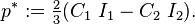
Cauchy stress in terms of principal stretches
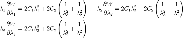
In terms of the principal stretches, the Cauchy stress differences for an incompressible hyperelastic material are given by

For an incompressible Mooney-Rivlin material,

Therefore,

Since  . we can write
Then the expressions for the Cauchy stress differences become

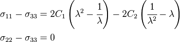
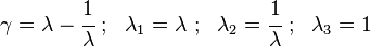
Uniaxial extension
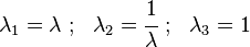
For the case of an incompressible Mooney–Rivlin material under uniaxial elongation,  and
and 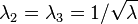 . Then the true stress (Cauchy stress) differences can be calculated as:
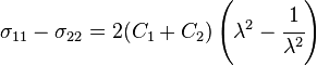
Simple tension

In the case of simple tension,  . Then we can write
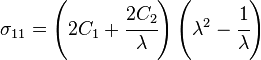
In alternative notation, where the Cauchy stress is written as  and the stretch as
  , we can write
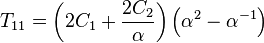
and the engineering stress (force per unit reference area) for an incompressible Mooney–Rivlin material under simple tension can be calculated using
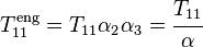 . Hence
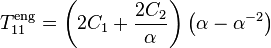
If we define
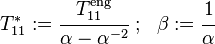
then
The slope of the  versus
  line gives the value of
  while the intercept with the axis gives the value of
  . The Mooney–Rivlin solid model usually fits experimental data better than Neo-Hookean solid does, but requires an additional empirical constant.
Equibiaxial tension
In the case of equibiaxial tension, the principal stretches are  . If, in addition, the material is incompressible then
  . The Cauchy stress differences may therefore be expressed as
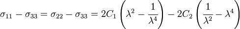
The equations for equibiaxial tension are equivalent to those governing uniaxial compression.
Pure shear
A pure shear deformation can be achieved by applying stretches of the form [7]
The Cauchy stress differences for pure shear may therefore be expressed as

Therefore
For a pure shear deformation

Therefore  .
.
Simple shear
The deformation gradient for a simple shear deformation has the form[7]
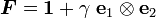
where  are reference orthonormal basis vectors in the plane of deformation and the shear deformation is given by
In matrix form, the deformation gradient and the left Cauchy-Green deformation tensor may then be expressed as
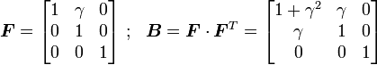
Therefore,
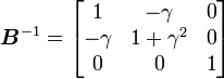
The Cauchy stress is given by
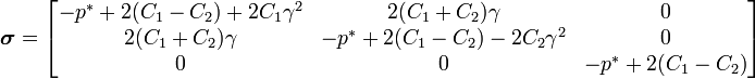
For consistency with linear elasticity, clearly 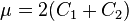 where is the shear modulus.
Rubber
Elastic response of rubber-like materials are often modeled based on the Mooney—Rivlin model. The constants  are determined by the fitting predicted stress from the above equations to experimental data. The recommended tests are uniaxial tension, equibiaxial compression, equibiaxial tension, uniaxial compression, and for shear, planar tension and planar compression. The two parameter Mooney–Rivlin model is usually valid for strains less than 100%.
Notes and references
- ↑ Mooney, M., 1940, A theory of large elastic deformation, Journal of Applied Physics, 11(9), pp. 582-592.
- ↑ Rivlin, R. S., 1948, Large elastic deformations of isotropic materials. IV. Further developments of the general theory, Philosophical Transactions of the Royal Society of London. Series A, Mathematical and Physical Sciences, 241(835), pp. 379-397.
- ↑ Boulanger, P. and Hayes, M. A., 2001, Finite amplitude waves in Mooney–Rivlin and Hadamard materials, in Topics in Finite Elasticity, ed. M. A Hayes and G. Soccomandi, International Center for Mechanical Sciences.
- ↑ C. W. Macosko, 1994, Rheology: principles, measurement and applications, VCH Publishers, ISBN 1-56081-579-5.
- ↑ The characteristic polynomial of the linear operator corresponding to the second rank three-dimensional Finger tensor (also called the left Cauchy–Green deformation tensor) is usually written
 is written , the next coefficient
  is written , and the determinant
  would be written
  .
. - ↑ Bower, Allan (2009). Applied Mechanics of Solids. CRC Press. ISBN 1-4398-0247-5. Retrieved January 2010.
- ↑ 7.0 7.1 Ogden, R. W., 1984, Nonlinear elastic deformations, Dover
