Modulational instability
In the fields of nonlinear optics and fluid dynamics, modulational instability or sideband instability is a phenomenon whereby deviations from a periodic waveform are reinforced by nonlinearity, leading to the generation of spectral-sidebands and the eventual breakup of the waveform into a train of pulses.[1][2][3]
The phenomenon was first discovered − and modelled − for periodic surface gravity waves (Stokes waves) on deep water by T. Brooke Benjamin and Jim E. Feir, in 1967.[4] Therefore, it is also known as the Benjamin−Feir instability. It is a possible mechanism for the generation of rogue waves.[5][6]
Initial instability and gain
Modulation instability only happens under certain circumstances. The most important condition is anomalous group velocity dispersion, whereby pulses with shorter wavelengths travel with higher group velocity than pulses with longer wavelength.[3] (This condition assumes a focussing Kerr nonlinearity, whereby refractive index increases with optical intensity.) There is also a threshold power, below which no instability will be seen.[3]
The instability is strongly dependent on the frequency of the perturbation. At certain frequencies, a perturbation will have little effect, whilst at other frequencies, a perturbation will grow exponentially. The overall gain spectrum can be derived analytically, as is shown below. Random perturbations will generally contain a broad range of frequency components, and so will cause the generation of spectral sidebands which reflect the underlying gain spectrum.
The tendency of a perturbing signal to grow makes modulation instability a form of amplification. By tuning an input signal to a peak of the gain spectrum, it is possible to create an optical amplifier.
Mathematical derivation of gain spectrum
The gain spectrum can be derived [3] by starting with a model of modulation instability based upon the Nonlinear Schrödinger equation

which describes the evolution of a slowly varying envelope  with time
  and distance of propagation
  . The model includes group velocity dispersion described by the parameter
  , and Kerr nonlinearity with magnitude
  . A waveform of constant power
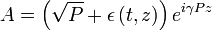
  is assumed. This is given by the solution

where the oscillatory  phase factor accounts for the difference between the linear refractive index, and the modified refractive index, as raised by the Kerr effect. The beginning of instability can be investigated by perturbing this solution as
where  is the perturbation term (which, for mathematical convenience, has been multiplied by the same phase factor as ). Substituting this back into the Nonlinear Schrödinger equation gives a perturbation equation of the form

where the perturbation has been assumed to be small, such that  . Instability can now be discovered by searching for solutions of the perturbation equation which grow exponentially. This can be done using a trial function of the general form

where  and
and  are the frequency and wavenumber of a perturbation, and
  and
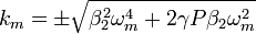
and  are constants. The Nonlinear Schrödinger equation is constructed by removing the carrier wave of the light being modelled, and so the frequency of the light being perturbed is formally zero. Therefore and don't represent absolute frequencies and wavenumbers, but the difference between these and those of the initial beam of light. It can be shown that the trial function is valid, subject to the condition
This dispersion relation is vitally dependent on the sign of the term within the square root, as if positive, the wavenumber will be real, corresponding to mere oscillations around the unperturbed solution, whilst if negative, the wavenumber will become imaginary, corresponding to exponential growth and thus instability. Therefore, instability will occur when
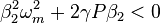
This condition describes both the requirement for anomalous dispersion (such that is negative) and the requirement that a threshold power be exceeded. The gain spectrum can be described by defining a gain parameter as 

![\Im\left[2|k_m|\right]](../I/m/0500431dd025e63f421a3d4df6dbf402.png) , so that the power of a perturbing signal grows with distance as
, so that the power of a perturbing signal grows with distance as 
 . The gain is therefore given by
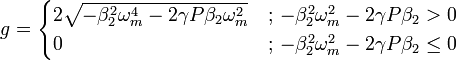
where as noted above, is the difference between the frequency of the perturbation and the frequency of the initial light.
Breakup
The waveform will eventually break up into a train of pulses.[3]
References
- ↑ Benjamin, T. Brooke; Feir, J.E. (1967). "The disintegration of wave trains on deep water. Part 1. Theory". Journal of Fluid Mechanics 27 (3): 417–430. Bibcode:1967JFM....27..417B. doi:10.1017/S002211206700045X.
- ↑ Benjamin, T.B. (1967). "Instability of Periodic Wavetrains in Nonlinear Dispersive Systems". Proceedings of the Royal Society of London. A. Mathematical and Physical Sciences 299 (1456): 59–76. Bibcode:1967RSPSA.299...59B. doi:10.1098/rspa.1967.0123. Concluded with a discussion by Klaus Hasselmann.
- ↑ 3.0 3.1 3.2 3.3 3.4 Agrawal, Govind P. (1995). Nonlinear fiber optics (2nd ed.). San Diego (California): Academic Press. ISBN 0-12-045142-5.
- ↑ Yuen, H.C.; Lake, B.M. (1980). "Instabilities of waves on deep water". Annual Review of Fluid Mechanics 12: 303–334. Bibcode:1980AnRFM..12..303Y. doi:10.1146/annurev.fl.12.010180.001511.
- ↑ Janssen, Peter A.E.M. (2003). "Nonlinear four-wave interactions and freak waves". Journal of Physical Oceanography 33 (4): 863–884. Bibcode:2003JPO....33..863J. doi:10.1175/1520-0485(2003)33<863:NFIAFW>2.0.CO;2.
- ↑ Dysthe, Kristian; Krogstad, Harald E.; Müller, Peter (2008). "Oceanic rogue waves". Annual Review of Fluid Mechanics 40: 287–310. Bibcode:2008AnRFM..40..287D. doi:10.1146/annurev.fluid.40.111406.102203.
Further reading
- Zakharov, V.E.; Ostrovsky, L.A. (2009). "Modulation instability: The beginning" (PDF). Physica D: Nonlinear Phenomena 238 (5): 540–548. Bibcode:2009PhyD..238..540Z. doi:10.1016/j.physd.2008.12.002.

| ||||||||||||||||||||||||||||