Modern portfolio theory

Modern portfolio theory (MPT) is a theory of finance that attempts to maximize portfolio expected return for a given amount of portfolio risk, or equivalently minimize risk for a given level of expected return, by carefully choosing the proportions of various assets. Although MPT is widely used in practice in the financial industry and several of its creators won a Nobel memorial prize for the theory,^[1] in recent years the basic assumptions of MPT have been widely challenged by fields such as behavioral economics.

MPT is a mathematical formulation of the concept of diversification in investing, with the aim of selecting a collection of investment assets that has collectively lower risk than any individual asset. This is possible, intuitively speaking, because different types of assets often change in value in opposite ways.^[2] For example, to the extent prices in the stock market move differently from prices in the bond market, a collection of both types of assets can in theory face lower overall risk than either individually. But diversification lowers risk even if assets' returns are not negatively correlated—indeed, even if they are positively correlated.^[3]

More technically, MPT models an asset's return as a normally or elliptically distributed random variable), defines risk as the standard deviation of return, and models a portfolio as a weighted combination of assets, so that the return of a portfolio is the weighted combination of the assets' returns. By combining different assets whose returns are not perfectly positively correlated, MPT seeks to reduce the total variance of the portfolio return. MPT also assumes that investors are rational and markets are efficient.

MPT was developed in the 1950s through the early 1970s and was considered an important advance in the mathematical modeling of finance. Since then, some theoretical and practical criticisms have been leveled against it. These include evidence that financial returns do not follow a Gaussian distribution or indeed any symmetric distribution, and that correlations between asset classes are not fixed but can vary depending on external events (especially in crises). Further, there remains evidence that investors are not rational and markets may not be efficient.^[4][5] Finally, the low volatility anomaly conflicts with CAPM's trade-off assumption of higher risk for higher return. It states that a portfolio consisting of low volatility equities (like blue chip stocks) reaps higher risk-adjusted returns than a portfolio with high volatility equities (like illiquid penny stocks). A study conducted by Myron Scholes, Michael Jensen, and Fischer Black in 1972 suggests that the relationship between return and beta might be flat or even negatively correlated.^[6]

Concept

The fundamental concept behind MPT is that the assets in an investment portfolio should not be selected individually, each on its own merits. Rather, it is important to consider how each asset changes in price relative to how every other asset in the portfolio changes in price.

Investing is a tradeoff between risk and expected return. In general, assets with higher expected returns are riskier. The stocks in an efficient portfolio are chosen depending on the investor's risk tolerance, an efficient portfolio is said to be having a combination of at least two stocks above the minimum variance portfolio. For a given amount of risk, MPT describes how to select a portfolio with the highest possible expected return. Or, for a given expected return, MPT explains how to select a portfolio with the lowest possible risk (the targeted expected return cannot be more than the highest-returning available security, of course, unless negative holdings of assets are possible.)^[7]

Therefore, MPT is a form of diversification. Under certain assumptions and for specific quantitative definitions of risk and return, MPT explains how to find the best possible diversification strategy.

History

Harry Markowitz introduced MPT in a 1952 article^[8] and a 1959 book.^[9] Markowitz classifies it simply as "Portfolio Theory," because "There's nothing modern about it." See also this^[7] survey of the history.

Mathematical model

In some sense the mathematical derivation below is MPT, although the basic concepts behind the model have also been very influential.^[7]

This section develops the "classic" MPT model. There have been many extensions since.

Risk and expected return

MPT assumes that investors are risk averse, meaning that given two portfolios that offer the same expected return, investors will prefer the less risky one. Thus, an investor will take on increased risk only if compensated by higher expected returns. Conversely, an investor who wants higher expected returns must accept more risk. The exact trade-off will be the same for all investors, but different investors will evaluate the trade-off differently based on individual risk aversion characteristics. The implication is that a rational investor will not invest in a portfolio if a second portfolio exists with a more favorable risk-expected return profile – i.e., if for that level of risk an alternative portfolio exists that has better expected returns.

Note that the theory uses standard deviation of return as a proxy for risk, which is valid if asset returns are jointly normally distributed or otherwise elliptically distributed. There are problems with this, however; see criticism.

Under the model:

• Portfolio return is the proportion-weighted combination of the constituent assets' returns.
• Portfolio volatility is a function of the correlations ρ_ij of the component assets, for all asset pairs (i, j).

In general:

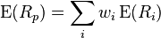
• Expected return:

where is the return on the portfolio, is the return on asset i and is the weighting of component asset (that is, the proportion of asset "i" in the portfolio).

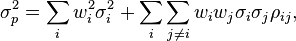
• Portfolio return variance:

where is the correlation coefficient between the returns on assets i and j. Alternatively the expression can be written as:

,

where for i=j.

• Portfolio return volatility (standard deviation):

For a two asset portfolio:

• Portfolio return:
• Portfolio variance:

For a three asset portfolio:

• Portfolio return:
• Portfolio variance:

Diversification

An investor can reduce portfolio risk simply by holding combinations of instruments that are not perfectly positively correlated (correlation coefficient ). In other words, investors can reduce their exposure to individual asset risk by holding a diversified portfolio of assets. Diversification may allow for the same portfolio expected return with reduced risk. These ideas have been started with Markowitz and then reinforced by other economists and mathematicians such as Andrew Brennan who have expressed ideas in the limitation of variance through portfolio theory.

If all the asset pairs have correlations of 0—they are perfectly uncorrelated—the portfolio's return variance is the sum over all assets of the square of the fraction held in the asset times the asset's return variance (and the portfolio standard deviation is the square root of this sum).

Efficient frontier with no risk-free asset

Efficient Frontier. The hyperbola is sometimes referred to as the 'Markowitz Bullet', and is the efficient frontier if no risk-free asset is available. With a risk-free asset, the straight line is the efficient frontier.

As shown in this graph, every possible combination of the risky assets, without including any holdings of the risk-free asset, can be plotted in risk-expected return space, and the collection of all such possible portfolios defines a region in this space. The left boundary of this region is a hyperbola,^[10] and the upper edge of this region is the efficient frontier in the absence of a risk-free asset (sometimes called "the Markowitz bullet"). Combinations along this upper edge represent portfolios (including no holdings of the risk-free asset) for which there is lowest risk for a given level of expected return. Equivalently, a portfolio lying on the efficient frontier represents the combination offering the best possible expected return for given risk level.

Matrices are preferred for calculations of the efficient frontier.

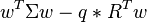
In matrix form, for a given "risk tolerance" , the efficient frontier is found by minimizing the following expression:

where

• is a vector of portfolio weights and (The weights can be negative, which means investors can short a security.);
• is the covariance matrix for the returns on the assets in the portfolio;
• is a "risk tolerance" factor, where 0 results in the portfolio with minimal risk and results in the portfolio infinitely far out on the frontier with both expected return and risk unbounded; and
• is a vector of expected returns.
• is the variance of portfolio return.
• is the expected return on the portfolio.

The above optimization finds the point on the frontier at which the inverse of the slope of the frontier would be q if portfolio return variance instead of standard deviation were plotted horizontally. The frontier in its entirety is parametric on q.

Many software packages, including MATLAB, Microsoft Excel, Mathematica and R, provide optimization routines suitable for the above problem.

An alternative approach to specifying the efficient frontier is to do so parametrically on the expected portfolio return This version of the problem requires that we minimize

subject to

for parameter . This problem is easily solved using a Lagrange multiplier.

Two mutual fund theorem

One key result of the above analysis is the two mutual fund theorem.^[10] This theorem states that any portfolio on the efficient frontier can be generated by holding a combination of any two given portfolios on the frontier; the latter two given portfolios are the "mutual funds" in the theorem's name. So in the absence of a risk-free asset, an investor can achieve any desired efficient portfolio even if all that is accessible is a pair of efficient mutual funds. If the location of the desired portfolio on the frontier is between the locations of the two mutual funds, both mutual funds will be held in positive quantities. If the desired portfolio is outside the range spanned by the two mutual funds, then one of the mutual funds must be sold short (held in negative quantity) while the size of the investment in the other mutual fund must be greater than the amount available for investment (the excess being funded by the borrowing from the other fund).

Risk-free asset and the capital allocation line

The risk-free asset is the (hypothetical) asset that pays a risk-free rate. In practice, short-term government securities (such as US treasury bills) are used as a risk-free asset, because they pay a fixed rate of interest and have exceptionally low default risk. The risk-free asset has zero variance in returns (hence is risk-free); it is also uncorrelated with any other asset (by definition, since its variance is zero). As a result, when it is combined with any other asset or portfolio of assets, the change in return is linearly related to the change in risk as the proportions in the combination vary.

When a risk-free asset is introduced, the half-line shown in the figure is the new efficient frontier. It is tangent to the hyperbola at the pure risky portfolio with the highest Sharpe ratio. Its vertical intercept represents a portfolio with 100% of holdings in the risk-free asset; the tangency with the hyperbola represents a portfolio with no risk-free holdings and 100% of assets held in the portfolio occurring at the tangency point; points between those points are portfolios containing positive amounts of both the risky tangency portfolio and the risk-free asset; and points on the half-line beyond the tangency point are leveraged portfolios involving negative holdings of the risk-free asset (the latter has been sold short—in other words, the investor has borrowed at the risk-free rate) and an amount invested in the tangency portfolio equal to more than 100% of the investor's initial capital. This efficient half-line is called the capital allocation line (CAL), and its formula can be shown to be

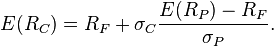
In this formula P is the sub-portfolio of risky assets at the tangency with the Markowitz bullet, F is the risk-free asset, and C is a combination of portfolios P and F.

By the diagram, the introduction of the risk-free asset as a possible component of the portfolio has improved the range of risk-expected return combinations available, because everywhere except at the tangency portfolio the half-line gives a higher expected return than the hyperbola does at every possible risk level. The fact that all points on the linear efficient locus can be achieved by a combination of holdings of the risk-free asset and the tangency portfolio is known as the one mutual fund theorem,^[10] where the mutual fund referred to is the tangency portfolio.

Asset pricing

The above analysis describes optimal behavior of an individual investor. Asset pricing theory builds on this analysis in the following way. Since everyone holds the risky assets in identical proportions to each other—namely in the proportions given by the tangency portfolio—in market equilibrium the risky assets' prices, and therefore their expected returns, will adjust so that the ratios in the tangency portfolio are the same as the ratios in which the risky assets are supplied to the market. Thus relative supplies will equal relative demands. MPT derives the required expected return for a correctly priced asset in this context.

Systematic risk and specific risk

Specific risk is the risk associated with individual assets - within a portfolio these risks can be reduced through diversification (specific risks "cancel out"). Specific risk is also called diversifiable, unique, unsystematic, or idiosyncratic risk. Systematic risk (a.k.a. portfolio risk or market risk) refers to the risk common to all securities—except for selling short as noted below, systematic risk cannot be diversified away (within one market). Within the market portfolio, asset specific risk will be diversified away to the extent possible. Systematic risk is therefore equated with the risk (standard deviation) of the market portfolio.

Since a security will be purchased only if it improves the risk-expected return characteristics of the market portfolio, the relevant measure of the risk of a security is the risk it adds to the market portfolio, and not its risk in isolation. In this context, the volatility of the asset, and its correlation with the market portfolio, are historically observed and are therefore given. (There are several approaches to asset pricing that attempt to price assets by modelling the stochastic properties of the moments of assets' returns - these are broadly referred to as conditional asset pricing models.)

Systematic risks within one market can be managed through a strategy of using both long and short positions within one portfolio, creating a "market neutral" portfolio. Market neutral portfolios, therefore will have a correlations of zero.

Capital asset pricing model

The asset return depends on the amount paid for the asset today. The price paid must ensure that the market portfolio's risk / return characteristics improve when the asset is added to it. The CAPM is a model that derives the theoretical required expected return (i.e., discount rate) for an asset in a market, given the risk-free rate available to investors and the risk of the market as a whole. The CAPM is usually expressed:

• , Beta, is the measure of asset sensitivity to a movement in the overall market; Beta is usually found via regression on historical data. Betas exceeding one signify more than average "riskiness" in the sense of the asset's contribution to overall portfolio risk; betas below one indicate a lower than average risk contribution.

• is the market premium, the expected excess return of the market portfolio's expected return over the risk-free rate.

The derivation is as follows:

(1) The incremental impact on risk and expected return when an additional risky asset, a, is added to the market portfolio, m, follows from the formulae for a two-asset portfolio. These results are used to derive the asset-appropriate discount rate.

• Market portfolio's risk =

Hence, risk added to portfolio =

but since the weight of the asset will be relatively low,

i.e. additional risk =

• Market portfolio's expected return =

Hence additional expected return =

(2) If an asset, a, is correctly priced, the improvement in its risk-to-expected return ratio achieved by adding it to the market portfolio, m, will at least match the gains of spending that money on an increased stake in the market portfolio. The assumption is that the investor will purchase the asset with funds borrowed at the risk-free rate, ; this is rational if .

Thus:

i.e. :

i.e. :

is the "beta", return— the covariance between the asset's return and the market's return divided by the variance of the market return— i.e. the sensitivity of the asset price to movement in the market portfolio's value.

This equation can be estimated statistically using the following regression equation:

where α_i is called the asset's alpha, β_i is the asset's beta coefficient and SCL is the security characteristic line.

Once an asset's expected return, , is calculated using CAPM, the future cash flows of the asset can be discounted to their present value using this rate to establish the correct price for the asset. A riskier stock will have a higher beta and will be discounted at a higher rate; less sensitive stocks will have lower betas and be discounted at a lower rate. In theory, an asset is correctly priced when its observed price is the same as its value calculated using the CAPM derived discount rate. If the observed price is higher than the valuation, then the asset is overvalued; it is undervalued for a too low price.

Criticisms

Despite its theoretical importance, critics of MPT question whether it is an ideal investing strategy, because its model of financial markets does not match the real world in many ways.^[11]

Efforts to translate the theoretical foundation into a viable portfolio construction algorithm have been plagued by technical difficulties stemming from the instability of the original optimization problem with respect to the available data. Recent research has shown that instabilities of this type disappear when a regularizing constraint or penalty term is incorporated in the optimization procedure.^[12]

Assumptions

The framework of MPT makes many assumptions about investors and markets. Some are explicit in the equations, such as the use of Normal distributions to model returns. Others are implicit, such as the neglect of taxes and transaction fees. None of these assumptions are entirely true, and each of them compromises MPT to some degree.

• Investors are interested in the optimization problem described above (maximizing the mean for a given variance). In reality, investors have utility functions that may be sensitive to higher moments of the distribution of the returns. For the investors to use the mean-variance optimization, one must suppose that the combination of utility and returns make the optimization of utility problem similar to the mean-variance optimization problem. A quadratic utility without any assumption about returns is sufficient. Another assumption is to use exponential utility and normal distribution, as discussed below.
• Asset returns are (jointly) normally distributed random variables. In fact, it is frequently observed that returns in equity and other markets are not normally distributed. Large swings (3 to 6 standard deviations from the mean) occur in the market far more frequently than the normal distribution assumption would predict.^[13] While the model can also be justified by assuming any return distribution that is jointly elliptical,^[14][15] all the joint elliptical distributions are symmetrical whereas asset returns empirically are not. Bouchaud and Chicheportiche (2012) ^[16] empirically reject the elliptical hypothesis, writing "intuitively, the failure of elliptical models can be traced to the inadequacy of the assumption of a single volatility model for all stocks."
• Correlations between assets are fixed and constant forever. Correlations depend on systemic relationships between the underlying assets, and change when these relationships change. Examples include one country declaring war on another, or a general market crash. During times of financial crisis all assets tend to become positively correlated, because they all move (down) together. In other words, MPT breaks down precisely when investors are most in need of protection from risk.
• All investors aim to maximize economic utility (in other words, to make as much money as possible, regardless of any other considerations). This is a key assumption of the efficient-market hypothesis, upon which MPT relies.
• All investors are rational and risk-averse. This is another assumption of the efficient-market hypothesis. In reality, as proven by behavioral economics, market participants are not always rational or consistently rational. The assumption does not account for emotional decisions, stale market information, "herd behavior", or investors who may seek risk for the sake of risk. Casino gamblers clearly pay for risk, and it is possible that some stock traders will pay for risk as well.
• All investors have access to the same information at the same time. In fact, real markets contain information asymmetry, insider trading, and those who are simply better informed than others. Moreover, estimating the mean (for instance, there is no consistent estimator of the drift of a brownian when subsampling between 0 and T) and the covariance matrix of the returns (when the number of assets is of the same order of the number of periods) are difficult statistical tasks.
• Investors have an accurate conception of possible returns, i.e., the probability beliefs of investors match the true distribution of returns. A different possibility is that investors' expectations are biased, causing market prices to be informationally inefficient. This possibility is studied in the field of behavioral finance, which uses psychological assumptions to provide alternatives to the CAPM such as the overconfidence-based asset pricing model of Kent Daniel, David Hirshleifer, and Avanidhar Subrahmanyam (2001).^[17]
• There are no taxes or transaction costs. Real financial products are subject both to taxes and transaction costs (such as broker fees), and taking these into account will alter the composition of the optimum portfolio. These assumptions can be relaxed with more complicated versions of the model.
• All investors are price takers, i.e., their actions do not influence prices. In reality, sufficiently large sales or purchases of individual assets can shift market prices for that asset and others (via cross elasticity of demand.) An investor may not even be able to assemble the theoretically optimal portfolio if the market moves too much while they are buying the required securities.
• Any investor can lend and borrow an unlimited amount at the risk free rate of interest. In reality, every investor has a credit limit.
• All securities can be divided into parcels of any size. In reality, fractional shares usually cannot be bought or sold, and some assets have minimum orders sizes.
• Risk/Volatility of an asset is known in advance/is constant. In fact, markets often misprice risk (e.g. the US mortgage bubble or the European debt crisis) and volatility changes rapidly.

More complex versions of MPT can take into account a more sophisticated model of the world (such as one with non-normal distributions and taxes) but all mathematical models of finance still rely on many unrealistic premises.

Poor model

The risk, return, and correlation measures used by MPT are based on expected values, which means that they are mathematical statements about the future (the expected value of returns is explicit in the above equations, and implicit in the definitions of variance and covariance). In practice, investors must substitute predictions based on historical measurements of asset return and volatility for these values in the equations. Very often such expected values fail to take account of new circumstances that did not exist when the historical data were generated.

More fundamentally, investors are stuck with estimating key parameters from past market data because MPT attempts to model risk in terms of the likelihood of losses, but says nothing about why those losses might occur. The risk measurements used are probabilistic in nature, not structural. This is a major difference as compared to many engineering approaches to risk management.

Options theory and MPT have at least one important conceptual difference from the probabilistic risk assessment done by nuclear power [plants]. A PRA is what economists would call a structural model. The components of a system and their relationships are modeled in Monte Carlo simulations. If valve X fails, it causes a loss of back pressure on pump Y, causing a drop in flow to vessel Z, and so on.

But in the Black–Scholes equation and MPT, there is no attempt to explain an underlying structure to price changes. Various outcomes are simply given probabilities. And, unlike the PRA, if there is no history of a particular system-level event like a liquidity crisis, there is no way to compute the odds of it. If nuclear engineers ran risk management this way, they would never be able to compute the odds of a meltdown at a particular plant until several similar events occurred in the same reactor design.

—Douglas W. Hubbard, 'The Failure of Risk Management', p. 67, John Wiley & Sons, 2009. ISBN 978-0-470-38795-5

Essentially, the mathematics of MPT view the markets as a collection of dice. By examining past market data we can develop hypotheses about how the dice are weighted, but this isn't helpful if the markets are actually dependent upon a much bigger and more complicated chaotic system—the world. For this reason, accurate structural models of real financial markets are unlikely to be forthcoming because they would essentially be structural models of the entire world. Nonetheless there is growing awareness of the concept of systemic risk in financial markets, which should lead to more sophisticated market models.

Mathematical risk measurements are also useful only to the degree that they reflect investors' true concerns—there is no point minimizing a variable that nobody cares about in practice. MPT uses the mathematical concept of variance to quantify risk, and this might be justified under the assumption of elliptically distributed returns such as normally distributed returns, but for general return distributions other risk measures (like coherent risk measures) might better reflect investors' true preferences.

In particular, variance is a symmetric measure that counts abnormally high returns as just as risky as abnormally low returns. Some would argue that, in reality, investors are only concerned about losses, and do not care about the dispersion or tightness of above-average returns. According to this view, our intuitive concept of risk is fundamentally asymmetric in nature.

MPT does not account for the personal, environmental, strategic, or social dimensions of investment decisions. It only attempts to maximize risk-adjusted returns, without regard to other consequences. In a narrow sense, its complete reliance on asset prices makes it vulnerable to all the standard market failures such as those arising from information asymmetry, externalities, and public goods. It also rewards corporate fraud and dishonest accounting. More broadly, a firm may have strategic or social goals that shape its investment decisions, and an individual investor might have personal goals. In either case, information other than historical returns is relevant.

Financial economist Nassim Nicholas Taleb has also criticized modern portfolio theory because it assumes a Gaussian distribution:

After the stock market crash (in 1987), they rewarded two theoreticians, Harry Markowitz and William Sharpe, who built beautifully Platonic models on a Gaussian base, contributing to what is called Modern Portfolio Theory. Simply, if you remove their Gaussian assumptions and treat prices as scalable, you are left with hot air. The Nobel Committee could have tested the Sharpe and Markowitz models—they work like quack remedies sold on the Internet—but nobody in Stockholm seems to have thought about it.

—^[18]:p.279

Effect on asset prices

Diversification eliminates non-systematic risk. As unsystematic risk is not associated with increased expected return, this is considered one of the few "free lunches" available. Following MPT means portfolio managers can invest in assets without analyzing their fundamentals, specially weighting each asset by the markets weight in the asset. Because the investor purchases assets in proportion to their market weights, there is no relative increase in demand for one asset versus another, and thus no impact on the expected returns of the portfolio.

Extensions

Since MPT's introduction in 1952, many attempts have been made to improve the model, especially by using more realistic assumptions.

Post-modern portfolio theory extends MPT by adopting non-normally distributed, asymmetric measures of risk. This helps with some of these problems, but not others.

Black-Litterman model optimization is an extension of unconstrained Markowitz optimization that incorporates relative and absolute `views' on inputs of risk and returns.

Other Applications

In the 1970s, concepts from Modern Portfolio Theory found their way into the field of regional science. In a series of seminal works, Michael Conroy modeled the labor force in the economy using portfolio-theoretic methods to examine growth and variability in the labor force. This was followed by a long literature on the relationship between economic growth and volatility.^[19]

More recently, modern portfolio theory has been used to model the self-concept in social psychology. When the self attributes comprising the self-concept constitute a well-diversified portfolio, then psychological outcomes at the level of the individual such as mood and self-esteem should be more stable than when the self-concept is undiversified. This prediction has been confirmed in studies involving human subjects.^[20]

Recently, modern portfolio theory has been applied to modelling the uncertainty and correlation between documents in information retrieval. Given a query, the aim is to maximize the overall relevance of a ranked list of documents and at the same time minimize the overall uncertainty of the ranked list.^[21]

Project portfolios and other "non-financial" assets

Some experts apply MPT to portfolios of projects and other assets besides financial instruments.^[22][23] When MPT is applied outside of traditional financial portfolios, some differences between the different types of portfolios must be considered.

1. The assets in financial portfolios are, for practical purposes, continuously divisible while portfolios of projects are "lumpy". For example, while we can compute that the optimal portfolio position for 3 stocks is, say, 44%, 35%, 21%, the optimal position for a project portfolio may not allow us to simply change the amount spent on a project. Projects might be all or nothing or, at least, have logical units that cannot be separated. A portfolio optimization method would have to take the discrete nature of projects into account.
2. The assets of financial portfolios are liquid; they can be assessed or re-assessed at any point in time. But opportunities for launching new projects may be limited and may occur in limited windows of time. Projects that have already been initiated cannot be abandoned without the loss of the sunk costs (i.e., there is little or no recovery/salvage value of a half-complete project).

Neither of these necessarily eliminate the possibility of using MPT and such portfolios. They simply indicate the need to run the optimization with an additional set of mathematically expressed constraints that would not normally apply to financial portfolios.

Furthermore, some of the simplest elements of Modern Portfolio Theory are applicable to virtually any kind of portfolio. The concept of capturing the risk tolerance of an investor by documenting how much risk is acceptable for a given return may be applied to a variety of decision analysis problems. MPT uses historical variance as a measure of risk, but portfolios of assets like major projects don't have a well-defined "historical variance". In this case, the MPT investment boundary can be expressed in more general terms like "chance of an ROI less than cost of capital" or "chance of losing more than half of the investment". When risk is put in terms of uncertainty about forecasts and possible losses then the concept is transferable to various types of investment.^[22]

Comparison with arbitrage pricing theory

The Security Market Line and capital asset pricing model are often contrasted with the arbitrage pricing theory (APT), which holds that the expected return of a financial asset can be modeled as a linear function of various macro-economic factors, where sensitivity to changes in each factor is represented by a factor specific beta coefficient.

The APT is less restrictive in its assumptions: it allows for a statistical model of asset returns, and assumes that each investor will hold a unique portfolio with its own particular array of betas, as opposed to the identical "market portfolio". Unlike the CAPM, the APT, however, does not itself reveal the identity of its priced factors—the number and nature of these factors is likely to change over time and between economies.

See also

• Bias ratio (finance)
• Black-Litterman model
• Fundamental analysis
• Intertemporal portfolio choice
• Investment theory
• Jensen's alpha
• Marginal conditional stochastic dominance
• Mutual fund separation theorem
• Omega ratio
• Post-modern portfolio theory
• Roll's critique
• Sortino ratio
• Treynor ratio
• Two-moment decision models
• Value investing
• Low-volatility anomaly

References

Further reading

• Lintner, John (1965). "The Valuation of Risk Assets and the Selection of Risky Investments in Stock Portfolios and Capital Budgets". The Review of Economics and Statistics (The MIT Press) 47 (1): 13–39. doi:10.2307/1924119. JSTOR 1924119. 
• Sharpe, William F. (1964). "Capital asset prices: A theory of market equilibrium under conditions of risk". Journal of Finance 19 (3): 425–442. doi:10.2307/2977928. JSTOR 2977928. 
• Tobin, James (1958). "Liquidity preference as behavior towards risk". The Review of Economic Studies 25 (2): 65–86. doi:10.2307/2296205. JSTOR 2296205. 

External links

• Macro-Investment Analysis, Prof. William F. Sharpe, Stanford University

References

- ↑ Harry M. Markowitz - Autobiography, The Nobel Prizes 1990, Editor Tore Frängsmyr, [Nobel Foundation], Stockholm, 1991
- ↑ "Managed Futures - Reducing Portfolio Volatility | A Look Into The Top 3 Managed Futures Accounts Worldwide". Emanagedfutures.com. 2011-03-19. Retrieved 2012-09-05.
- ↑ Bhalla, V. K. (2010). Investment Management. New Delhi: S. Chand & Co. Ltd. pp. 587–93. ISBN 81-219-1248-2.
- ↑ Andrei Shleifer: Inefficient Markets: An Introduction to Behavioral Finance. Clarendon Lectures in Economics (2000)
- ↑ Koponen, Timothy M. 2003. Commodities in action: measuring embeddedness and imposing values. The Sociological Review. Volume 50 Issue 4, Pages 543 - 569
- ↑ Jenson, Michael; Scholes, Myron; Black, Fischer (1972). "The Capital Asset Pricing Model: Some Empirical Tests". In Jensen, Michael. Studies in the Theory of Capital Markets. Praeger Publishers. Retrieved 2014-03-24.
- ↑ 7.0 7.1 7.2 Edwin J. Elton and Martin J. Gruber, "Modern portfolio theory, 1950 to date", Journal of Banking & Finance 21 (1997) 1743-1759
- ↑ Markowitz, H.M. (March 1952). "Portfolio Selection". The Journal of Finance 7 (1): 77–91. doi:10.2307/2975974. JSTOR 2975974.
- ↑ Markowitz, H.M. (1959). Portfolio Selection: Efficient Diversification of Investments. New York: John Wiley & Sons. (reprinted by Yale University Press, 1970, ISBN 978-0-300-01372-6; 2nd ed. Basil Blackwell, 1991, ISBN 978-1-55786-108-5)
- ↑ 10.0 10.1 10.2 Merton, Robert. "An analytic derivation of the efficient portfolio frontier," Journal of Financial and Quantitative Analysis 7, September 1972, 1851-1872.
- ↑ Mahdavi Damghani B. (2013). "The Non-Misleading Value of Inferred Correlation: An Introduction to the Cointelation Model". Wilmott Magazine. doi:10.1002/wilm.10252.
- ↑ Brodie, De Mol, Daubechies, Giannone and Loris (2009). "Sparse and stable Markowitz portfolios". Proceedings of the National Academy of Sciences 106 (30). doi:10.1073/pnas.0904287106.
- ↑ Mandelbrot, B., and Hudson, R. L. (2004). The (Mis)Behaviour of Markets: A Fractal View of Risk, Ruin, and Reward. London: Profile Books.
- ↑ Chamberlain, G. 1983."A characterization of the distributions that imply mean-variance utility functions", Journal of Economic Theory 29, 185-201.
- ↑ Owen, J.; Rabinovitch, R. (1983). "On the class of elliptical distributions and their applications to the theory of portfolio choice". Journal of Finance 38: 745–752. doi:10.1111/j.1540-6261.1983.tb02499.x.
- ↑ http://arxiv.org/pdf/1009.1100.pdf Chicheportiche, R., & Bouchaud, J. P. (2012). The joint distribution of stock returns is not elliptical. International Journal of Theoretical and Applied Finance, 15(03).
- ↑ 'Overconfidence, Arbitrage, and Equilibrium Asset Pricing,' Kent D. Daniel, David Hirshleifer and Avanidhar Subrahmanyam, Journal of Finance, 56(3) (June, 2001), pp. 921-965
- ↑ Taleb, Nassim Nicholas (2007), The Black Swan: The Impact of the Highly Improbable, Random House, ISBN 978-1-4000-6351-2.
- ↑ Chandra, Siddharth (2003). "Regional Economy Size and the Growth-Instability Frontier: Evidence from Europe". Journal of Regional Science 43 (1): 95–122. doi:10.1111/1467-9787.00291.
- ↑ Chandra, Siddharth; Shadel, William G. (2007). "Crossing disciplinary boundaries: Applying financial portfolio theory to model the organization of the self-concept". Journal of Research in Personality 41 (2): 346–373. doi:10.1016/j.jrp.2006.04.007.
- ↑ Portfolio Theory of Information Retrieval July 11th, 2009 (2009-07-11). "Portfolio Theory of Information Retrieval | Dr. Jun Wang's Home Page". Web4.cs.ucl.ac.uk. Retrieved 2012-09-05.
- ↑ 22.0 22.1 Hubbard, Douglas (2007). How to Measure Anything: Finding the Value of Intangibles in Business. Hoboken, NJ: John Wiley & Sons. ISBN 978-0-470-11012-6.
- ↑ Sabbadini, Tony (2010). "Manufacturing Portfolio Theory" (PDF). International Institute for Advanced Studies in Systems Research and Cybernetics.