Meshfree methods
In the field of numerical simulation methods, meshfree methods are those that do not require that a mesh connect data points of the simulation domain. Meshfree methods enable the simulation of some otherwise difficult types of problems, at the cost of extra computing time and programming effort.
Motivation
Numerical methods such as the finite difference method, finite-volume method, and finite element method were originally defined on meshes of data points. In such a mesh, each point has a fixed number of predefined neighbors, and this connectivity between neighbors can be used to define mathematical operators like the derivative. These operators are then used to construct the equations to simulate—such as the Euler equations or the Navier–Stokes equations.
But in simulations where the material being simulated can move around (as in computational fluid dynamics) or where large deformations of the material can occur (as in simulations of plastic materials), the connectivity of the mesh can be difficult to maintain without introducing error into the simulation. If the mesh becomes tangled or degenerate during simulation, the operators defined on it may no longer give correct values. The mesh may be recreated during simulation (a process called remeshing), but this can also introduce error, since all the existing data points must be mapped onto a new and different set of data points. Meshfree methods are intended to remedy these problems. Meshfree methods are also useful for:
- Simulations where creating a useful mesh from the geometry of a complex 3D object may be especially difficult or require human assistance
- Simulations where nodes may be created or destroyed, such as in cracking simulations
- Simulations where the problem geometry may move out of alignment with a fixed mesh, such as in bending simulations
- Simulations containing nonlinear material behavior, discontinuities or singularities
Example
In a traditional finite difference simulation, the domain of a one-dimensional simulation would be some function  , represented as a mesh of data values
  at points
  , where


We can define the derivatives that occur in the equation being simulated using some finite difference formulae on this domain, for example
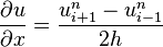
and
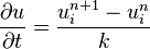
Then we can use these definitions of and its spatial and temporal derivatives to write the equation being simulated in finite difference form, then simulate the equation with one of many finite difference methods.
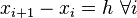
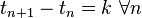
In this simple example, the spatial step size  and the temporal step size
  are constant, and the left and right mesh neighbors of the data value at are the values at
  and
and  , respectively. But if the values can move around, or can be added to or removed from the simulation, that destroys the spacing and the simple finite difference formulae for derivatives is no longer correct.
Smoothed-particle hydrodynamics (SPH), one of the oldest meshfree methods, solves this problem by treating data points as physical particles with mass and density that can move around over time, and carry some value  with them. SPH then defines the value of between the particles by
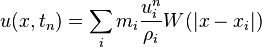
where  is the mass of particle
  ,
,  is the density of particle , and
  is a kernel function that operates on nearby data points and is chosen for smoothness and other useful qualities. By linearity, we can write the spatial derivative as
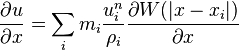
Then we can use these definitions of and its spatial derivatives to write the equation being simulated as an ordinary differential equation, and simulate the equation with one of many numerical methods. In physical terms, this means calculating the forces between the particles, then integrating these forces over time to determine their motion.
The advantage of SPH in this situation is that the formulae for and its derivatives do not depend on any adjacency information about the particles; they can use the particles in any order, so it doesn't matter if the particles move around or even exchange places.
One disadvantage of SPH is that it requires extra programming to determine the nearest neighbors of a particle. Since the kernel function only returns nonzero results for nearby particles within twice the "smoothing length" (because we typically choose kernel functions with compact support), it would be a waste of effort to calculate the summations above over every particle in a large simulation. So typically SPH simulators require some extra code to speed up this nearest neighbor calculation.
History
One of the earliest meshfree methods is smoothed particle hydrodynamics, presented in 1977.[1] Over the ensuing decades, many more methods have been developed, some of which are listed below.
List of methods and acronyms
The following numerical methods are generally considered to fall within the general class of "meshfree" methods. Acronyms are provided in parentheses.
- Smoothed particle hydrodynamics (SPH) (1977)
- Diffuse element method (DEM) (1992)
- Dissipative particle dynamics (DPD) (1992)
- Element-free Galerkin method (EFG / EFGM) (1994)
- Reproducing kernel particle method (RKPM) (1995)
- Finite pointset method (FPM) (1998)
- hp-clouds
- Natural element method (NEM)
- Material point method (MPM)
- Meshless local Petrov Galerkin (MLPG)
- Moving particle semi-implicit (MPS)
- Generalized finite difference method (GFDM)
- Particle-in-cell (PIC)
- Moving particle finite element method (MPFEM)
- Finite cloud method (FCM)
- Boundary node method (BNM)
- Meshfree moving Kriging interpolation method (MK)
- Boundary cloud method (BCM)
- Method of fundamental solution(MFS)
- Method of particular solution (MPS)
- Method of finite spheres (MFS)
- Discrete vortex method (DVM)
- Finite mass method (FMM) (2000)[2]
- Smoothed point interpolation method (S-PIM) (2005).[3]
- Meshfree local radial point interpolation method (RPIM).[3]
- Local radial basis function collocation Method (LRBFCM)[4]
- Viscous vortex domains method (VVD)
- Discrete least squares meshless method (DLSM) (2006)
- Repeated replacement method (RRM) (2012)[5]
- Radial basis integral equation method[6]
Related methods:
- Moving least squares (MLS) – provide general approximation method for arbitrary set of nodes
- Partition of unity methods (PoUM) – provide general approximation formulation used in some meshfree methods
- Continuous blending method (enrichment and coupling of finite elements and meshless methods) – see Huerta & Fernández-Méndez (2000)
- eXtended FEM, Generalized FEM (XFEM, GFEM) – variants of FEM (finite element method) combining some meshless aspects
- Smoothed finite element method (S-FEM) (2007)
- Gradient smoothing method (GSM) (2008)
- Local maximum-entropy (LME) – see Arroyo & Ortiz (2006)
- Space-Time Meshfree Collocation Method (STMCM) – see Netuzhylov (2008), Netuzhylov & Zilian (2009)
Recent development
One recent advance in meshfree methods aim at the development of computational tools for automation in modeling and simulations. This is enabled by the so-called weakened weak (W2) formulation based on the G space theory.[7] The W2 formulation offers possibilities for formulate various (uniformly) "soft" models that works well with triangular meshes. Because triangular mesh can be generated automatically, it becomes much easier in re-meshing and hence automation in modeling and simulation. In addition, W2 models can be made soft enough (in uniform fashion) to produce upper bound solutions (for force-driving problems). Together with stiff models (such as the fully compatible FEM models), one can conveniently bound the solution from both sides. This allows easy error estimation for generally complicated problems, as long as a triangular mesh can be generated. Typical W2 models are the Smoothed Point Interpolation Methods (or S-PIM).[3] The S-PIM can be node-based (known as NS-PIM or LC-PIM),[8] edge-based (ES-PIM),[9] and cell-based (CS-PIM).[10] The NS-PIM was developed using the so-called SCNI technique.[11] It was then discovered that NS-PIM is capable of producing upper bound solution and volumetric locking free.[12] The ES-PIM is found superior in accuracy, and CS-PIM behaves in between the NS-PIM and ES-PIM. Moreover, W2 formulations allow the use of polynomial and radial basis functions in the creation of shape functions (it accommodates the discontinuous displacement functions, as long as it is in G1 space), which opens further rooms for future developments.
The W2 formulation has also led to the development of combination of meshfree techniques with the well-developed FEM techniques, and one can now use triangular mesh with excellent accuracy and desired softness. A typical such a formulation is the so-called Smoothed Finite Element Method (or S-FEM) [13] The S-FEM is the linear version of S-PIM, but with most of the properties of the S-PIM and much simpler.
It is a general perception that meshfree methods are much more expensive than the FEM counterparts. The recent study has found however, the S-PIM and S-FEM can be much faster than the FEM counterparts.[3][13]
The S-PIM and S-FEM works well for solid mechanics problems. For [CFD] problems, the formulation can be simpler, via strong formulation. A Gradient Smoothing Methods (GSM) has also been developed recently for [CFD] problems, implementing the gradient smoothing idea in strong form.[14][15] The GSM is similar to [FVM], but uses gradient smoothing operations exclusively in nested fashions, and is a general numerical method for PDEs.
Nodal integration has been proposed as a technique to use finite elements to emulate a meshfree behaviour.[16] However, the obstacle that must be overcome in using nodally integrated elements is that the quantities at nodal points are not continuous, and the nodes are shared among multiple elements.
See also
- Continuum mechanics
- Smoothed finite element method[13]
- G space[17]
- Weakened weak form[7]
- Boundary element method
- Immersed boundary method
- Stencil code
References
- ↑ Gingold RA, Monaghan JJ (1977). Smoothed particle hydrodynamics – theory and application to non-spherical stars. Mon Not R Astron Soc 181:375–389
- ↑ C. Gauger, P. Leinen, H. Yserentant The finite mass method. SIAM J. Numer. Anal. 37 (2000), 176
- ↑ 3.0 3.1 3.2 3.3 Liu, G.R. 2nd edn: 2009 Mesh Free Methods, CRC Press. 978-1-4200-8209-9
- ↑ Sarler B, Vertnik R. Meshfree
- ↑ Walker WA (2012) The Repeated Replacement Method: A Pure Lagrangian Meshfree Method for Computational Fluid Dynamics. PLoS ONE 7(7): e39999. doi:10.1371/journal.pone.0039999
- ↑ Ooi EH, Popov V (2012) An efficient implementation of the radial basis integral equation method. Engineering Analysis with Boundary Elements, 36: 716-726
- ↑ 7.0 7.1 G.R. Liu. A G space theory and a weakened weak (W2) form for a unified formulation of compatible and incompatible methods: Part I theory and Part II applications to solid mechanics problems. International Journal for Numerical Methods in Engineering, 81: 1093–1126, 2010
- ↑ Liu GR, Zhang GY, Dai KY, Wang YY, Zhong ZH, Li GY and Han X, A linearly conforming point interpolation method (LC-PIM) for 2D solid mechanics problems, International Journal of Computational Methods, 2(4): 645–665, 2005.
- ↑ G.R. Liu, G.R. Zhang. Edge-based Smoothed Point Interpolation Methods. International Journal of Computational Methods, 5(4): 621–646, 2008
- ↑ G.R. Liu, G.R. Zhang. A normed G space and weakened weak (W2) formulation of a cell-based Smoothed Point Interpolation Method. International Journal of Computational Methods, 6(1): 147–179, 2009
- ↑ Chen, J. S., Wu, C. T., Yoon, S. and You, Y. (2001). A stabilized conforming nodal integration for Galerkin mesh-free methods. Int. J. Numer. Meth. Eng. 50: 435–466.
- ↑ G. R. Liu and G. Y. Zhang. Upper bound solution to elasticity problems: A unique property of the linearly conforming point interpolation method (LC-PIM). International Journal for Numerical Methods in Engineering, 74: 1128–1161, 2008.
- ↑ 13.0 13.1 13.2 Liu, G.R., 2010 Smoothed Finite Element Methods, CRC Press, ISBN 978-1-4398-2027-8.
- ↑ G. R. Liu, George X. Xu. A gradient smoothing method (GSM) for fluid dynamics problems. International Journal for Numerical Methods in Fluids, 58: 1101–1133, 2008.
- ↑ J. Zhang, G. R. Liu, K.Y. Lam, H. Li, G. Xu. A gradient smoothing method (GSM) based on strong form governing equation for adaptive analysis of solid mechanics problems. Finite Elements in Analysis and Design, 44: 889–909, 2008.
- ↑ Simoes, D. A.; Jadhav, T. A. (January 2014). "Nodally Integrated Finite Element Formulation for Mindlin-Reissner Plates". International Journal of Scientific & Engineering Research 5 (1): 1977–1982. Bibcode:2014IJSER...5.1977S. doi:10.14299/ijser.2014.01.001. ISSN 2229-5518. Retrieved 3 March 2014.
- ↑ Liu GR, ON G SPACE THEORY, INTERNATIONAL JOURNAL OF COMPUTATIONAL METHODS, Vol. 6 Issue: 2,257-289, 2009
Further reading
- Liu MB, Liu GR, Zong Z, AN OVERVIEW ON SMOOTHED PARTICLE HYDRODYNAMICS, INTERNATIONAL JOURNAL OF COMPUTATIONAL METHODS Vol. 5 Issue: 1, 135–188, 2008.
- Liu, G.R., Liu, M.B. (2003). Smoothed Particle Hydrodynamics, a meshfree and Particle Method, World Scientific, ISBN 981-238-456-1.
- Atluri, S.N. (2004), "The Meshless Method (MLPG) for Domain & BIE Discretization", Tech Science Press. ISBN 0-9657001-8-6
- Arroyo, M.; Ortiz, M. (2006), "Local maximum-entropy approximation schemes: a seamless bridge between finite elements and meshfree methods", International Journal for Numerical Methods in Engineering 65 (13): 2167–2202, Bibcode:2006IJNME..65.2167A, doi:10.1002/nme.1534.
- Belytschko, T., Chen, J.S. (2007). Meshfree and Particle Methods, John Wiley and Sons Ltd. ISBN 0-470-84800-6
- Belytschko, T.; Huerta, A.; Fernández-Méndez, S; Rabczuk, T. (2004), "Meshless methods", Encyclopedia of computational mechanics vol. 1 Chapter 10, John Wiley & Sons. ISBN 0-470-84699-2
- Liu, G.R. 1st edn, 2002. Mesh Free Methods, CRC Press. ISBN 0-8493-1238-8.
- Li, S., Liu, W.K. (2004). Meshfree Particle Methods, Berlin: Springer Verlag. ISBN 3-540-22256-1
- Huerta, A.; Fernández-Méndez, S. (2000), "Enrichment and coupling of the finite element and meshless methods", International Journal for Numerical Methods in Engineering 11 (11): 1615–1636, Bibcode:2000IJNME..48.1615H, doi:10.1002/1097-0207(20000820)48:11<1615::AID-NME883>3.0.CO;2-S.
- Netuzhylov, H. (2008), "A Space-Time Meshfree Collocation Method for Coupled Problems on Irregularly-Shaped Domains", Dissertation, TU Braunschweig, CSE – Computational Sciences in Engineering ISBN 978-3-00-026744-4, also as electronic ed..
- Netuzhylov, H.; Zilian, A. (2009), "Space-time meshfree collocation method: methodology and application to initial-boundary value problems", International Journal for Numerical Methods in Engineering 80 (3): 355–380, Bibcode:2009IJNME..80..355N, doi:10.1002/nme.2638
- Alhuri. Y, A. Naji, D. Ouazar and A. Taik. (2010). RBF Based Meshless Method for Large Scale Shallow Water Simulations: Experimental Validation, Math. Model. Nat. Phenom, Vol. 5, No. 7, 2010, pp. 4–10.
- P. L. Machado, R. M. S. de Oliveira, W. C. B. Souza, R. C. F. Araújo, M. E. L. Tostes, and C. Gonçalves. (2011). An Automatic Methodology for Obtaining Optimum Shape Factors for the Radial Point Interpolation Method, Journal of Microwaves, Optoelectronics and Electromagnetic Applications, Vol. 10, No. 2, 2011, pp. 389-401.
External links
- The first available commercial fully automated meshfree structural analysis solution
- The first available commercial meshfree CFD code
- The USACM blog on Meshfree Methods