Mellin transform
In mathematics, the Mellin transform is an integral transform that may be regarded as the multiplicative version of the two-sided Laplace transform. This integral transform is closely connected to the theory of Dirichlet series, and is often used in number theory, mathematical statistics, and the theory of asymptotic expansions; it is closely related to the Laplace transform and the Fourier transform, and the theory of the gamma function and allied special functions.
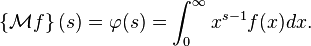
The Mellin transform of a function f is
The inverse transform is
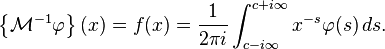
The notation implies this is a line integral taken over a vertical line in the complex plane. Conditions under which this inversion is valid are given in the Mellin inversion theorem.
The transform is named after the Finnish mathematician Hjalmar Mellin.
Relationship to other transforms
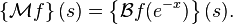
The two-sided Laplace transform may be defined in terms of the Mellin transform by

and conversely we can get the Mellin transform from the two-sided Laplace transform by
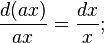
The Mellin transform may be thought of as integrating using a kernel xs with respect to the multiplicative Haar measure,
 , which is invariant
under dilation
, which is invariant
under dilation  , so that
 the two-sided Laplace transform integrates with respect to the additive Haar measure
  , which is translation invariant, so that
  .
.
We also may define the Fourier transform in terms of the Mellin transform and vice versa; if we define the two-sided Laplace transform as above, then

We may also reverse the process and obtain

The Mellin transform also connects the Newton series or binomial transform together with the Poisson generating function, by means of the Poisson–Mellin–Newton cycle.
Examples
Cahen–Mellin integral
For  ,
,  and
and  on the principal branch, one has
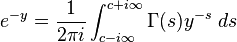
where  is the gamma function. This integral is known as the Cahen-Mellin integral.[1]
Number theory
An important application in number theory includes the simple function 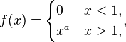 for which
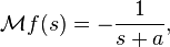
assuming
As a unitary operator on L2
In the study of Hilbert spaces, the Mellin transform is often posed in a slightly different way. For functions in  (see Lp space) the fundamental strip always includes
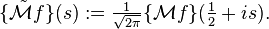
  , so we may define a linear operator
  as
as

In other words we have set
This operator is usually denoted by just plain  and called the "Mellin transform", but is used here to distinguish from the definition used elsewhere in this article. The Mellin inversion theorem then shows that is invertible with inverse

Furthermore this operator is an isometry, that is to say 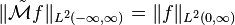 for all
  (this explains why the factor of
  was used). Thus is a unitary operator.
In probability theory
In probability theory, the Mellin transform is an essential tool in studying the distributions of products of random variables.[2] If X is a random variable, and X+ = max{X,0} denotes its positive part, while X − = max{−X,0} is its negative part, then the Mellin transform of X is defined as [3]
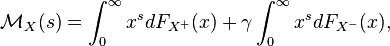
where γ is a formal indeterminate with γ2 = 1. This transform exists for all s in some complex strip D = {s: a ≤ Re(s) ≤ b}, where a ≤ 0 ≤ b.[3]
The Mellin transform  of a random variable X uniquely determines its distribution function FX.[3] The importance of the Mellin transform in probability theory lies in the fact that if X and Y are two independent random variables, then the Mellin transform of their products is equal to the product of the Mellin transforms of X and Y:[4]

In cylindrical problems with laplacian
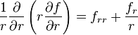
In the Laplacian in cylindrical coordinates in a generic dimension (orthogonal coordinates with one angle and one radius, and the remaining lengths) there is always a term:
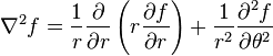
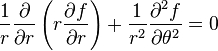
For example in 2-D polar coordinates the laplacian is:
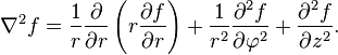
and in 3-D cylindrical coordinates the laplacian is,
This term can be easily treated with the Mellin transform,[5] since:

For example the 2-D Laplace equation in polar coordinates is the PDE in two variables:
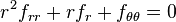
and by multiplication:
with a Mellin transform on radius becomes the simple harmonic oscillator:
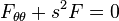
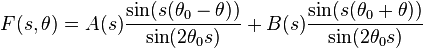
with general solution:

Now let's impose for example some simple wedge boundary conditions to the original Laplace equation:

these are particularly simple for Mellin transform, becoming:
 .
.
These conditions imposed to the solution particularise it to:
Now by the convolution theorem for Mellin transform, the solution in the Mellin domain can be inverted:

where the following inverse transform relation was employed:
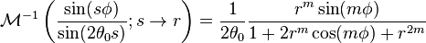
where  .
.
Applications
The Mellin Transform is widely used in computer science for the analysis of algorithms because of its scale invariance property. The magnitude of the Mellin Transform of a scaled function is identical to the magnitude of the original function. This scale invariance property is analogous to the Fourier Transform's shift invariance property. The magnitude of a Fourier transform of a time-shifted function is identical to the magnitude of the Fourier transform of the original function.
This property is useful in image recognition. An image of an object is easily scaled when the object is moved towards or away from the camera.
Examples
- Perron's formula describes the inverse Mellin transform applied to a Dirichlet series.
- The Mellin transform is used in analysis of the prime-counting function and occurs in discussions of the Riemann zeta function.
- Inverse Mellin transforms commonly occur in Riesz means.
- The Mellin transform can be used in Audio timescale-pitch modification (needs substantive reference).
See also
Notes
- ↑ Hardy, G. H.; Littlewood, J. E. (1916). "Contributions to the Theory of the Riemann Zeta-Function and the Theory of the Distribution of Primes". Acta Mathematica 41 (1): 119–196. doi:10.1007/BF02422942. (See notes therein for further references to Cahen's and Mellin's work, including Cahen's thesis.)
- ↑ Galambos & Simonelli (2004, p. 15)
- ↑ 3.0 3.1 3.2 Galambos & Simonelli (2004, p. 16)
- ↑ Galambos & Simonelli (2004, p. 23)
- ↑ Bhimsen, Shivamoggi, Chapter 6: The Mellin Transform, par. 4.3: Distribution of a Potential in a Wedge, p. 267-8
References
- Galambos, Janos; Simonelli, Italo (2004). Products of random variables: applications to problems of physics and to arithmetical functions. Marcel Dekker, Inc. ISBN 0-8247-5402-6.
- Paris, R. B.; Kaminski, D. (2001). Asymptotics and Mellin-Barnes Integrals. Cambridge University Press.
- Polyanin, A. D.; Manzhirov, A. V. (1998). Handbook of Integral Equations. Boca Raton: CRC Press. ISBN 0-8493-2876-4.
- Flajolet, P.; Gourdon, X.; Dumas, P. (1995). "Mellin transforms and asymptotics: Harmonic sums". Theoretical Computer Science 144 (1-2): 3–58. doi:10.1016/0304-3975(95)00002-e.
- Tables of Integral Transforms at EqWorld: The World of Mathematical Equations.
- Hazewinkel, Michiel, ed. (2001), "Mellin transform", Encyclopedia of Mathematics, Springer, ISBN 978-1-55608-010-4
- Weisstein, Eric W., "Mellin Transform", MathWorld.
External links
- Philippe Flajolet, Xavier Gourdon, Philippe Dumas, Mellin Transforms and Asymptotics: Harmonic sums.
- Antonio Gonzáles, Marko Riedel Celebrando un clásico, newsgroup es.ciencia.matematicas
- Juan Sacerdoti, Funciones Eulerianas (in Spanish).
- Mellin Transform Methods, Digital Library of Mathematical Functions, 2011-08-29, National Institute of Standards and Technology
- Antonio De Sena and Davide Rocchesso, A FAST MELLIN TRANSFORM WITH APPLICATIONS IN DAFX