Mean difference

Not to be confused with Median absolute deviation.

The mean difference is a measure of statistical dispersion equal to the average absolute difference of two independent values drawn from a probability distribution. A related statistic is the relative mean difference, which is the mean difference divided by the arithmetic mean. An important relationship is that the relative mean difference is equal to twice the Gini coefficient, which is defined in terms of the Lorenz curve.

The mean difference is also known as the absolute mean difference and the Gini mean difference. The mean difference is sometimes denoted by Δ or as MD. The mean deviation is a different measure of dispersion.

Definition

The mean difference is defined as the "average" or "mean", formally the expected value, of the absolute difference of two random variables X and Y independently and identically distributed with the same (unknown) distribution henceforth called Q.

\mathrm{MD} := E[|X - Y|] .

Calculation

Specifically,

if Q has a discrete probability function f(y), where y_i, i = 1 to n, are the values with nonzero probabilities:

\mathrm{MD} = \Sigma_{i=1}^n \Sigma_{j=1}^n f(y_i) f(y_j) | y_i - y_j | .

if Q has a probability density function f(x):

\mathrm{MD} = \int_{-\infty}^\infty \int_{-\infty}^\infty f(x)\,f(y)\,|x-y|\,dx\,dy .

if Q has a cumulative distribution function F(x) with quantile function F(x):

\mathrm{MD} = \int_0^1 \int_0^1 |F(x)-F(y)|\,dx\,dy .

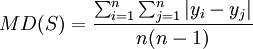
For a random sample of size n of a population distributed according to Q, the (empirical) mean difference of the sequence of sample values y_i, i = 1 to n can be caluated as the arithmetic mean of the absolute value of all possible differences:

\mathrm{MD} = \frac{1}{n^2} \Sigma_{i=1}^n \Sigma_{j=1}^n | y_i - y_j | .

Relative mean difference

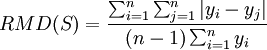
When the probability distribution has a finite and nonzero arithmetic mean, the relative mean difference, sometimes denoted by ∇ or RMD, is defined by

RMD = \frac{MD}{\mbox{arithmetic mean}}.

The relative mean difference quantifies the mean difference in comparison to the size of the mean and is a dimensionless quantity. The relative mean difference is equal to twice the Gini coefficient which is defined in terms of the Lorenz curve. This relationship gives complementary perspectives to both the relative mean difference and the Gini coefficient, including alternative ways of calculating their values.

Properties

The mean difference is invariant to translations and negation, and varies proportionally to positive scaling. That is to say, if X is a random variable and c is a constant:

MD(X + c) = MD(X),
MD(-X) = MD(X), and
MD(c X) = |c| MD(X).

The relative mean difference is invariant to positive scaling, commutes with negation, and varies under translation in proportion to the ratio of the original and translated arithmetic means. That is to say, if X is a random variable and c is a constant:

RMD(X + c) = RMD(X) · mean(X)/(mean(X) + c) = RMD(X) / (1+c / mean(X)) for c ≠ -mean(X),
RMD(-X) = −RMD(X), and
RMD(c X) = RMD(X) for c > 0.

If a random variable has a positive mean, then its relative mean difference will always be greater than or equal to zero. If, additionally, the random variable can only take on values that are greater than or equal to zero, then its relative mean difference will be less than 2.

Compared to standard deviation

The mean difference is twice the L-scale (the second L-moment), while the standard deviation is the square root of the variance about the mean (the second conventional central moment). The differences between L-moments and conventional moments are first seen in comparing the mean difference and the standard deviation (the first L-moment and first conventional moment are both the mean).

Both the standard deviation and the mean difference measure dispersion—how spread out are the values of a population or the probabilities of a distribution. The mean difference is not defined in terms of a specific measure of central tendency, whereas the standard deviation is defined in terms of the deviation from the arithmetic mean. Because the standard deviation squares its differences, it tends to give more weight to larger differences and less weight to smaller differences compared to the mean difference. When the arithmetic mean is finite, the mean difference will also be finite, even when the standard deviation is infinite. See the examples for some specific comparisons.

The recently introduced distance standard deviation plays similar role to the mean difference but the distance standard deviation works with centered distances. See also E-statistics.

Sample estimators

For a random sample S from a random variable X, consisting of n values y_i, the statistic

MD(S) = \frac{\sum_{i=1}^n \sum_{j=1}^n | y_i - y_j |}{n(n-1)}

is a consistent and unbiased estimator of MD(X). The statistic:

RMD(S) = \frac{\sum_{i=1}^n \sum_{j=1}^n | y_i - y_j |}{(n-1)\sum_{i=1}^n y_i}

is a consistent estimator of RMD(X), but is not, in general, unbiased.

Confidence intervals for RMD(X) can be calculated using bootstrap sampling techniques.

There does not exist, in general, an unbiased estimator for RMD(X), in part because of the difficulty of finding an unbiased estimation for multiplying by the inverse of the mean. For example, even where the sample is known to be taken from a random variable X(p) for an unknown p, and X(p) - 1 has the Bernoulli distribution, so that Pr(X(p) = 1) = 1 − p and Pr(X(p) = 2) = p, then

RMD(X(p)) = 2p(1 − p)/(1 + p).

But the expected value of any estimator R(S) of RMD(X(p)) will be of the form:

\operatorname{E}(R(S)) = \sum_{i=0}^n p^i (1-p)^{n-i} r_i ,

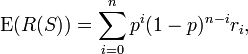
where the r _i are constants. So E(R(S)) can never equal RMD(X(p)) for all p between 0 and 1.

Examples

Examples of Mean Difference and Relative Mean Difference
Distribution	Parameters	Mean	Standard Deviation	Mean Difference	Relative Mean Difference
Continuous uniform	a = 0 ; b = 1	1 / 2 = 0.5	$\frac{1}{\sqrt{12}}$ ≈ 0.2887	1 / 3 ≈ 0.3333	2 / 3 ≈ 0.6667
Normal	μ = 1 ; σ = 1	1	1	$\frac{2}{\sqrt{\pi}}$ ≈ 1.1284	$\frac{2}{\sqrt{\pi}}$ ≈ 1.1284
Exponential	λ = 1	1	1	1	1
Pareto	k > 1 ; x_m = 1	$\frac{k}{(k-1)}$	$\frac{1}{(k-1)}\,\sqrt{\frac{k}{(k-2)}}$ (for k > 2)	$\frac{2 k} {(k-1) (2k-1)} \,$	$\frac{2}{2k-1}\,$
Gamma	k ; θ	kθ	$\sqrt{k}\,\theta$	k θ (2 − 4 I_0.5(k+1 , k)) †	2 − 4 I_0.5(k+1 , k) †
Gamma	k = 1 ; θ = 1	1	1	1	1
Gamma	k = 2 ; θ = 1	2	$\sqrt{2}$ ≈ 1.4142	3 / 2 = 1.5	3 / 4 = 0.75
Gamma	k = 3 ; θ = 1	3	$\sqrt{3}$ ≈ 1.7321	15 / 8 = 1.875	5 / 8 = 0.625
Gamma	k = 4 ; θ = 1	4	2	35 / 16 = 2.1875	35 / 64 = 0.546875
Bernoulli	0 ≤ p ≤ 1	p	$\sqrt{p(1-p)}$	2 p (1 − p)	2 (1 − p) for p > 0
Student's t, 2 d.f.	ν = 2	0	$\infty$	π / √2 = 2.2214	undefined

† I_z(x,y) is the regularized incomplete Beta function

References

Xu, Kuan (January 2004). "How Has the Literature on Gini's Index Evolved in the Past 80 Years?". Department of Economics, Dalhousie University. Retrieved 2006-06-01.
Gini, Corrado (1912). Variabilità e Mutabilità. Bologna: Tipografia di Paolo Cuppini.
Gini, Corrado (1921). "Measurement of Inequality and Incomes". The Economic Journal (The Economic Journal, Vol. 31, No. 121) 31 (121): 124–126. doi:10.2307/2223319. JSTOR 2223319.
Chakravarty, S. R. (1990). Ethical Social Index Numbers. New York: Springer-Verlag.
Mills, Jeffrey A.; Zandvakili, Sourushe (1997). "Statistical Inference via Bootstrapping for Measures of Inequality". Journal of Applied Econometrics 12 (2): 133–150. doi:10.1002/(SICI)1099-1255(199703)12:2<133::AID-JAE433>3.0.CO;2-H.
Lomnicki, Z. A. (1952). "The Standard Error of Gini's Mean Difference". Annals of Mathematical Statistics 23 (4): 635–637. doi:10.1214/aoms/1177729346.
Nair, U. S. (1936). "Standard Error of Gini's Mean Difference". Biometrika 28: 428–436. doi:10.1093/biomet/28.3-4.428.
Yitzhaki, Shlomo (2003). "Gini's Mean difference: a superior measure of variability for non-normal distributions". Metron - International Journal of Statistics 61: 285–316.