Maxwell's equations

For thermodynamic relations, see Maxwell relations. For the history of the equations, see History of Maxwell's equations.

Electromagnetism

Electricity Magnetism
Electrostatics Electric charge Static electricity Electric field Conductor Insulator Triboelectricity Electrostatic discharge Induction Coulomb's law Gauss's law Electric flux / potential energy Electric dipole moment Polarization density
Magnetostatics Ampère's law Magnetic field Magnetization Magnetic flux Biot–Savart law Magnetic dipole moment Gauss's law for magnetism
Electrodynamics Lorentz force law Electromagnetic induction Faraday's law Lenz's law Displacement current Maxwell's equations Electromagnetic field Electromagnetic radiation Maxwell tensor Poynting vector Liénard–Wiechert potential Jefimenko's equations Eddy current London equations
Electrical network Electric current Electric potential Voltage Resistance Ohm's law Series circuit Parallel circuit Direct current Alternating current Charged current Neutral current Electromotive force Capacitance Inductance Impedance Resonant cavities Waveguides
Covariant formulation Electromagnetic tensor (stress–energy tensor) Four-current Electromagnetic four-potential
Scientists Ampère Coulomb Faraday Gauss Heaviside Henry Hertz Lorentz Maxwell Tesla Volta Weber Ørsted

Maxwell's equations are a set of partial differential equations that, together with the Lorentz force law, form the foundation of classical electrodynamics, classical optics, and electric circuits. These fields in turn underlie modern electrical and communications technologies. Maxwell's equations describe how electric and magnetic fields are generated and altered by each other and by charges and currents. They are named after the Scottish physicist and mathematician James Clerk Maxwell, who published an early form of those equations between 1861 and 1862.

The equations have two major variants. The "microscopic" set of Maxwell's equations uses total charge and total current, including the complicated charges and currents in materials at the atomic scale; it has universal applicability but may be infeasible to calculate. The "macroscopic" set of Maxwell's equations defines two new auxiliary fields that describe large-scale behaviour without having to consider these atomic scale details, but it requires the use of parameters characterizing the electromagnetic properties of the relevant materials.

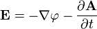
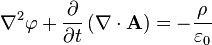
The term "Maxwell's equations" is often used for other forms of Maxwell's equations. For example, space-time formulations are commonly used in high energy and gravitational physics. These formulations, defined on space-time rather than space and time separately, are manifestly^{[note 1]} compatible with special and general relativity. In quantum mechanics and analytical mechanics, versions of Maxwell's equations based on the electric and magnetic potentials are preferred.

Since the mid-20th century, it has been understood that Maxwell's equations are not exact laws of the universe, but are a classical approximation to the more accurate and fundamental theory of quantum electrodynamics. In most cases, though, quantum deviations from Maxwell's equations are immeasurably small. Exceptions occur when the particle nature of light is important or for very strong electric fields.

Formulation in terms of electric and magnetic fields

The powerful and most widely familiar form of Maxwell's equations, whose formulation is due to Oliver Heaviside, in the vector calculus formalism, is used throughout unless otherwise explicitly stated.

Symbols in bold represent vector quantities, and symbols in italics represent scalar quantities, unless otherwise indicated.

The equations introduce the electric field $E$ , a vector field, and the magnetic field $B$ , a pseudovector field, where each generally have time-dependence. The sources of these fields are electric charges and electric currents, which can be expressed as local densities namely charge density $ρ$ and current density $J$ . A separate law of nature, the Lorentz force law, describes how the electric and magnetic field act on charged particles and currents. A version of this law was included in the original equations by Maxwell but, by convention, is no longer.

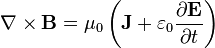
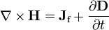
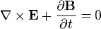
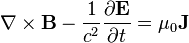
In the electric-magnetic field formulation there are four equations. Two of them describe how the fields vary in space due to sources, if any; electric fields emanating from electric charges in Gauss's law, and magnetic fields as closed field lines not due to magnetic monopoles in Gauss's law for magnetism. The other two describe how the fields "circulate" around their respective sources; the magnetic field "circulates" around electric currents and time varying electric fields in Ampère's law with Maxwell's addition, while the electric field "circulates" around time varying magnetic fields in Faraday's law.

The precise formulation of Maxwell's equations depends on the precise definition of the quantities involved. Conventions differ with the unit systems, because various definitions and dimensions are changed by absorbing dimensionful factors like the speed of light $c$ . This makes constants come out differently.

Conventional formulation in SI units

The equations in this section are given in the convention used with SI units. Other units commonly used are Gaussian units based on the cgs system,^[1] Lorentz–Heaviside units (used mainly in particle physics), and Planck units (used in theoretical physics). See below for the formulation with Gaussian units.

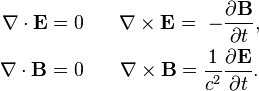
Name	Integral equations	Differential equations
Gauss's law	$\oiint$ ${\scriptstyle\partial \Omega }$ $\mathbf{E}\cdot\mathrm{d}\mathbf{S} = \frac{1}{\varepsilon_0} \iiint_\Omega \rho \,\mathrm{d}V$	$\nabla \cdot \mathbf{E} = \frac {\rho} {\varepsilon_0}$
Gauss's law for magnetism	$\oiint$ ${\scriptstyle \partial \Omega }$ $\mathbf{B}\cdot\mathrm{d}\mathbf{S} = 0$	$\nabla \cdot \mathbf{B} = 0$
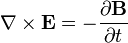
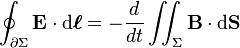
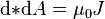
Maxwell–Faraday equation (Faraday's law of induction)	$\oint_{\partial \Sigma} \mathbf{E} \cdot \mathrm{d}\boldsymbol{\ell} = - \frac{d}{dt} \iint_{\Sigma} \mathbf{B} \cdot \mathrm{d}\mathbf{S}$	$\nabla \times \mathbf{E} = -\frac{\partial \mathbf{B}} {\partial t}$
Ampère's circuital law (with Maxwell's addition)	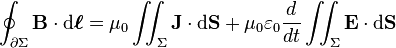$\oint_{\partial \Sigma} \mathbf{B} \cdot \mathrm{d}\boldsymbol{\ell} = \mu_0 \iint_{\Sigma} \mathbf{J} \cdot \mathrm{d}\mathbf{S} + \mu_0 \varepsilon_0 \frac{d}{dt} \iint_{\Sigma} \mathbf{E} \cdot \mathrm{d}\mathbf{S}$	$\nabla \times \mathbf{B} = \mu_0\left(\mathbf{J} + \varepsilon_0 \frac{\partial \mathbf{E}} {\partial t} \right)$

where the universal constants appearing in the equations are

the permittivity of free space $ε 0$ and
the permeability of free space $μ 0$ .

In the differential equations, a local description of the fields,

the nabla symbol $\nabla$ denotes the three-dimensional gradient operator, and from it
the divergence operator is $\nabla \cdot$
the curl operator is $\nabla \times$ .

The sources are taken to be

the electric charge density (charge per unit volume) $ρ$ and
the electric current density (current per unit area) $J$ .

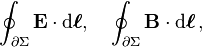
In the integral equations, a description of the fields within a region of space,

$Ω$ is any fixed volume with boundary surface $\partialΩ$ , and
$Σ$ is any fixed open surface with boundary curve $\partialΣ$ ,
$\oiint$ ${\scriptstyle\partial \Omega }$ is a surface integral over the surface $\partialΩ$ (the oval indicates the surface is closed and not open),
$\iiint_\Omega$ is a volume integral over the volume $Ω$ ,
$\iint_\Sigma$ is a surface integral over the surface $Σ$ ,
$\oint_{\partial \Sigma}$ is a line integral around the curve $\partialΣ$ (the circle indicates the curve is closed).

Here "fixed" means the volume or surface do not change in time. Although it is possible to formulate Maxwell's equations with time-dependent surfaces and volumes, this is not actually necessary: the equations are correct and complete with time-independent surfaces. The sources are correspondingly the total amounts of charge and current within these volumes and surfaces, found by integration.

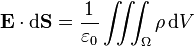
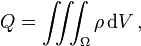
The volume integral of the total charge density $ρ$ over any fixed volume $Ω$ is the total electric charge contained in $Ω$ :

Q = \iiint_\Omega \rho \, \mathrm{d}V\,,

where

dV

is the differential volume element, and

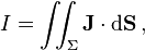
the net electrical current is the surface integral of the electric current density $J$ , passing through any open fixed surface $Σ$ :

I = \iint_{\Sigma} \mathbf{J} \cdot \mathrm{d} \mathbf{S}\,,

where

d S

denotes the differential vector element of surface area

S

normal to surface

Σ

. (Vector area is also denoted by

A

rather than

S

, but this conflicts with the magnetic potential, a separate vector field).

The "total charge or current" refers to including free and bound charges, or free and bound currents. These are used in the macroscopic formulation below.

Relationship between differential and integral formulations

The differential and integral formulations of the equations are mathematically equivalent, by the divergence theorem in the case of Gauss's law and Gauss's law for magnetism, and by the Kelvin–Stokes theorem in the case of Faraday's law and Ampère's law. Both the differential and integral formulations are useful. The integral formulation can often be used to simplify and directly calculate fields from symmetric distributions of charges and currents. On the other hand, the differential formulation is a more natural starting point for calculating the fields in more complicated (less symmetric) situations, for example using finite element analysis.^[2]

Flux and divergence

Closed volume

Ω

and its boundary

\partialΩ

, enclosing a source

(+)

and sink

(-)

of a vector field

F

. Here,

F

could be the

E

field with source electric charges, but not the

B

field which has no magnetic charges as shown. The outward unit normal is n.

The "fields emanating from the sources" can be inferred from the surface integrals of the fields through the closed surface $\partialΩ$ , defined as the electric flux $\oiint$ ${\scriptstyle \partial \Omega }$ $\mathbf{E}\cdot\mathrm{d}\mathbf{S}$ and magnetic flux $\oiint$ ${\scriptstyle \partial \Omega }$ $\mathbf{B}\cdot\mathrm{d}\mathbf{S}$ , as well as their respective divergences $\nabla \cdot E$ and $\nabla \cdot B$ . These surface integrals and divergences are connected by the divergence theorem.

Circulation and curl

Open surface

Σ

and boundary

\partialΣ

F

could be the

E

B

fields. Again,

n

is the unit normal. (The curl of a vector field doesn't literally look like the "circulations", this is a heuristic depiction).

The "circulation of the fields" can be interpreted from the line integrals of the fields around the closed curve ∂Σ:

\oint_{\partial \Sigma} \mathbf{E} \cdot \mathrm{d}\boldsymbol{\ell}, \quad \oint_{\partial \Sigma} \mathbf{B} \cdot \mathrm{d}\boldsymbol{\ell}\,,

where $d ℓ$ is the differential vector element of path length tangential to the path/curve, as well as their curls:

\nabla \times \mathbf{E}, \quad \nabla \times \mathbf{B}\,.

These line integrals and curls are connected by Stokes' theorem, and are analogous to quantities in classical fluid dynamics: the circulation of a fluid is the line integral of the fluid's flow velocity field around a closed loop, and the vorticity of the fluid is the curl of the velocity field.

Time evolution

The "dynamics" or "time evolution of the fields" is due to the partial derivatives of the fields with respect to time:

\frac{\partial\mathbf{E}}{\partial t}, \quad \frac{\partial\mathbf{B}}{\partial t}.

These derivatives are crucial for the prediction of field propagation in the form of electromagnetic waves. Since the surface is taken to be time-independent, we can make the following transition in Faraday's law:

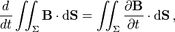
\frac{d}{dt} \iint_{\Sigma} \mathbf{B} \cdot \mathrm{d}\mathbf{S} = \iint_{\Sigma} \frac{\partial \mathbf{B}}{\partial t} \cdot \mathrm{d}\mathbf{S}\,,

see differentiation under the integral sign for more on this result.

Conceptual descriptions

Gauss's law

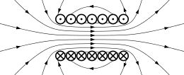
Gauss's law describes the relationship between a static electric field and the electric charges that cause it: The static electric field points away from positive charges and towards negative charges. In the field line description, electric field lines begin only at positive electric charges and end only at negative electric charges. 'Counting' the number of field lines passing through a closed surface, therefore, yields the total charge (including bound charge due to polarization of material) enclosed by that surface divided by dielectricity of free space (the vacuum permittivity). More technically, it relates the electric flux through any hypothetical closed "Gaussian surface" to the enclosed electric charge.

Gauss's law for magnetism: magnetic field lines never begin nor end but form loops or extend to infinity as shown here with the magnetic field due to a ring of current.

Gauss's law for magnetism

Gauss's law for magnetism states that there are no "magnetic charges" (also called magnetic monopoles), analogous to electric charges.^[3] Instead, the magnetic field due to materials is generated by a configuration called a dipole. Magnetic dipoles are best represented as loops of current but resemble positive and negative 'magnetic charges', inseparably bound together, having no net 'magnetic charge'. In terms of field lines, this equation states that magnetic field lines neither begin nor end but make loops or extend to infinity and back. In other words, any magnetic field line that enters a given volume must somewhere exit that volume. Equivalent technical statements are that the sum total magnetic flux through any Gaussian surface is zero, or that the magnetic field is a solenoidal vector field.

Faraday's law

In a geomagnetic storm, a surge in the flux of charged particles temporarily alters Earth's magnetic field, which induces electric fields in Earth's atmosphere, thus causing surges in electrical power grids. Artist's rendition; sizes are not to scale.

The Maxwell-Faraday's equation version of Faraday's law describes how a time varying magnetic field creates ("induces") an electric field.^[3] This dynamically induced electric field has closed field lines just as the magnetic field, if not superposed by a static (charge induced) electric field. This aspect of electromagnetic induction is the operating principle behind many electric generators: for example, a rotating bar magnet creates a changing magnetic field, which in turn generates an electric field in a nearby wire.

Ampère's law with Maxwell's addition

Magnetic core memory (1954) is an application of Ampère's law. Each core stores one bit of data.

Ampère's law with Maxwell's addition states that magnetic fields can be generated in two ways: by electrical current (this was the original "Ampère's law") and by changing electric fields (this was "Maxwell's addition").

Maxwell's addition to Ampère's law is particularly important: it shows that not only does a changing magnetic field induce an electric field, but also a changing electric field induces a magnetic field.^[3]^[4] Therefore, these equations allow self-sustaining "electromagnetic waves" to travel through empty space (see electromagnetic wave equation).

The speed calculated for electromagnetic waves, which could be predicted from experiments on charges and currents,^{[note 2]} exactly matches the speed of light; indeed, light is one form of electromagnetic radiation (as are X-rays, radio waves, and others). Maxwell understood the connection between electromagnetic waves and light in 1861, thereby unifying the theories of electromagnetism and optics.

Vacuum equations, electromagnetic waves and speed of light

Further information: Electromagnetic wave equation, Inhomogeneous electromagnetic wave equation and Sinusoidal plane-wave solutions of the electromagnetic wave equation

This 3D diagram shows a plane linearly polarized wave propagating from left to right with the same wave equations where

E = E 0 sin(-ω t + k \cdot r)

and

B = B 0 sin(-ω t + k \cdot r)

In a region with no charges ( $ρ = 0$ ) and no currents ( $J = 0$ ), such as in a vacuum, Maxwell's equations reduce to:

\begin{align} \nabla \cdot \mathbf{E} &= 0 \quad &\nabla \times \mathbf{E} = \ -&\frac{\partial\mathbf B}{\partial t}, \\ \nabla \cdot \mathbf{B} &= 0 \quad &\nabla \times \mathbf{B} = \frac{1}{c^2} &\frac{\partial \mathbf E}{\partial t}. \end{align}

Taking the curl $(\nabla\times)$ of the curl equations, and using the curl of the curl identity $\nabla\times(\nabla\times X) = \nabla(\nabla\cdot X) - \nabla 2 X$ we obtain the wave equations

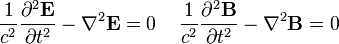
\frac{1}{c^2}\frac{\partial^2 \mathbf E}{\partial t^2} - \nabla^2 \mathbf E = 0\, \quad \frac{1}{c^2}\frac{\partial^2 \mathbf B}{\partial t^2} - \nabla^2 \mathbf B = 0\,

which identify

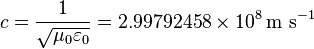
c = \frac{1}{\sqrt{ \mu_0 \varepsilon_0}} = 2.99792458 \times 10^8 \, \mathrm{m~s}^{-1}

with the speed of light in free space. In materials with relative permittivity $ε r$ and relative permeability $μ r$ , the phase velocity of light becomes

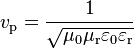
v_\text{p} = \frac{1}{\sqrt{ \mu_0\mu_\text{r} \varepsilon_0\varepsilon_\text{r} }}

which is usually less than $c$ .

In addition, $E$ and $B$ are mutually perpendicular to each other and the direction of wave propagation, and are in phase with each other. A sinusoidal plane wave is one special solution of these equations. Maxwell's equations explain how these waves can physically propagate through space. The changing magnetic field creates a changing electric field through Faraday's law. In turn, that electric field creates a changing magnetic field through Maxwell's addition to Ampère's law. This perpetual cycle allows these waves, now known as electromagnetic radiation, to move through space at velocity $c$ .

"Microscopic" versus "macroscopic"

The microscopic variant of Maxwell's equation expresses the electric $E$ field and the magnetic $B$ field in terms of the total charge and total current present including the charges and currents at the atomic level. It is sometimes called the general form of Maxwell's equations or "Maxwell's equations in a vacuum". The macroscopic variant of Maxwell's equation is equally general, however, with the difference being one of bookkeeping.

"Maxwell's macroscopic equations", also known as Maxwell's equations in matter, are more similar to those that Maxwell introduced himself.

Name	Integral equations	Differential equations
Gauss's law	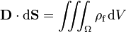$\oiint$ ${\scriptstyle \partial \Omega }$ $\mathbf{D}\cdot\mathrm{d}\mathbf{S} = \iiint_\Omega \rho_\text{f} \,\mathrm{d}V$	$\nabla \cdot \mathbf{D} = \rho_\text{f}$
Gauss's law for magnetism	$\oiint$ ${\scriptstyle \partial \Omega }$ $\mathbf{B}\cdot\mathrm{d}\mathbf{S} = 0$	$\nabla \cdot \mathbf{B} = 0$
Maxwell–Faraday equation (Faraday's law of induction)	$\oint_{\partial \Sigma} \mathbf{E} \cdot \mathrm{d}\boldsymbol{\ell} = - \frac{d}{dt} \iint_{\Sigma} \mathbf B \cdot \mathrm{d}\mathbf{S}$	$\nabla \times \mathbf{E} = -\frac{\partial \mathbf{B}} {\partial t}$
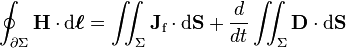
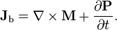
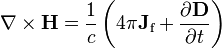
Ampère's circuital law (with Maxwell's addition)	$\oint_{\partial \Sigma} \mathbf{H} \cdot \mathrm{d}\boldsymbol{\ell} = \iint_{\Sigma} \mathbf{J}_\text{f} \cdot \mathrm{d}\mathbf{S} + \frac{d}{dt} \iint_{\Sigma} \mathbf{D} \cdot \mathrm{d}\mathbf{S}$	$\nabla \times \mathbf{H} = \mathbf{J}_\text{f} + \frac{\partial \mathbf{D}} {\partial t}$

Unlike the "microscopic" equations, the "macroscopic" equations separate out the bound charge $Q b$ and current $I b$ to obtain equations that depend only on the free charges $Q f$ and currents $I f$ . This factorization can be made by splitting the total electric charge and current as follows:

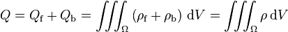
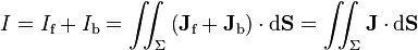
Q = Q_\text{f} + Q_\text{b} = \iiint_\Omega \left(\rho_\text{f} + \rho_\text{b} \right) \, \mathrm{d}V = \iiint_\Omega \rho \,\mathrm{d}V

I = I_\text{f} + I_\text{b} = \iint_\Sigma \left(\mathbf{J}_\text{f} + \mathbf{J}_\text{b} \right) \cdot \mathrm{d}\mathbf{S} = \iint_\Sigma \mathbf{J} \cdot \mathrm{d}\mathbf{S}

Correspondingly, the total current density $J$ splits into free $J f$ and bound $J b$ components, and similarly the total charge density $ρ$ splits into free $ρ f$ and bound $ρ b$ parts.

The cost of this factorization is that additional fields, the displacement field $D$ and the magnetizing field $H$ , are defined and need to be determined. Phenomenological constituent equations relate the additional fields to the electric field $E$ and the magnetic $B$ -field, often through a simple linear relation.

For a detailed description of the differences between the microscopic (total charge and current including material contributes or in air/vacuum)^{[note 3]} and macroscopic (free charge and current; practical to use on materials) variants of Maxwell's equations, see below.

Bound charge and current

Main articles: Current density, Bound charge and Bound current

Left: A schematic view of how an assembly of microscopic dipoles produces opposite surface charges as shown at top and bottom. Right: How an assembly of microscopic current loops add together to produce a macroscopically circulating current loop. Inside the boundaries, the individual contributions tend to cancel, but at the boundaries no cancelation occurs.

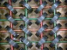
When an electric field is applied to a dielectric material its molecules respond by forming microscopic electric dipoles – their atomic nuclei move a tiny distance in the direction of the field, while their electrons move a tiny distance in the opposite direction. This produces a macroscopic bound charge in the material even though all of the charges involved are bound to individual molecules. For example, if every molecule responds the same, similar to that shown in the figure, these tiny movements of charge combine to produce a layer of positive bound charge on one side of the material and a layer of negative charge on the other side. The bound charge is most conveniently described in terms of the polarization $P$ of the material, its dipole moment per unit volume. If $P$ is uniform, a macroscopic separation of charge is produced only at the surfaces where $P$ enters and leaves the material. For non-uniform $P$ , a charge is also produced in the bulk.^[5]

Somewhat similarly, in all materials the constituent atoms exhibit magnetic moments that are intrinsically linked to the angular momentum of the components of the atoms, most notably their electrons. The connection to angular momentum suggests the picture of an assembly of microscopic current loops. Outside the material, an assembly of such microscopic current loops is not different from a macroscopic current circulating around the material's surface, despite the fact that no individual charge is traveling a large distance. These bound currents can be described using the magnetization $M$ .^[6]

The very complicated and granular bound charges and bound currents, therefore, can be represented on the macroscopic scale in terms of $P$ and $M$ which average these charges and currents on a sufficiently large scale so as not to see the granularity of individual atoms, but also sufficiently small that they vary with location in the material. As such, Maxwell's macroscopic equations ignore many details on a fine scale that can be unimportant to understanding matters on a gross scale by calculating fields that are averaged over some suitable volume.

Auxiliary fields, polarization and magnetization

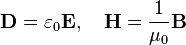
The definitions (not constitutive relations) of the auxiliary fields are:

\mathbf{D}(\mathbf{r}, t) = \varepsilon_0 \mathbf{E}(\mathbf{r}, t) + \mathbf{P}(\mathbf{r}, t)

\mathbf{H}(\mathbf{r}, t) = \frac{1}{\mu_0} \mathbf{B}(\mathbf{r}, t) - \mathbf{M}(\mathbf{r}, t),

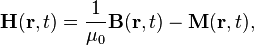
where $P$ is the polarization field and $M$ is the magnetization field which are defined in terms of microscopic bound charges and bound currents respectively. The macroscopic bound charge density $ρ b$ and bound current density $J b$ in terms of polarization $P$ and magnetization $M$ are then defined as

\rho_\text{b} = -\nabla\cdot\mathbf{P},

\mathbf{J}_\text{b} = \nabla\times\mathbf{M} + \frac{\partial\mathbf{P}}{\partial t}.

If we define the free, bound, and total charge and current density by

\rho = \rho_\text{b} + \rho_\text{f}, \

\mathbf{J} = \mathbf{J}_\text{b} + \mathbf{J}_\text{f},

and use the defining relations above to eliminate $D$ , and $H$ , the "macroscopic" Maxwell's equations reproduce the "microscopic" equations.

Constitutive relations

Main article: Constitutive equation § Electromagnetism

In order to apply 'Maxwell's macroscopic equations', it is necessary to specify the relations between displacement field $D$ and the electric field $E$ , as well as the magnetizing field $H$ and the magnetic field $B$ . Equivalently, we have to specify the dependence of the polarisation $P$ (hence the bound charge) and the magnetisation $M$ (hence the bound current) on the applied electric and magnetic field. The equations specifying this response are called constitutive relations. For real-world materials, the constitutive relations are rarely simple, except approximately, and usually determined by experiment. See the main article on constitutive relations for a fuller description.

For materials without polarisation and magnetisation ("vacuum"), the constitutive relations are

\mathbf{D} = \varepsilon_0\mathbf{E}, \quad \mathbf{H} = \frac{1}{\mu_0}\mathbf{B}

for scalar constants $ε 0$ and $μ 0$ . Since there is no bound charge, the total and the free charge and current are equal.

More generally, for linear materials the constitutive relations are

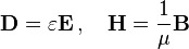
\mathbf{D} = \varepsilon\mathbf{E}\,,\quad \mathbf{H} = \frac{1}{\mu}\mathbf{B}

where $ε$ is the permittivity and $μ$ the permeability of the material. Even the linear case can have various complications, however.

For homogeneous materials, $ε$ and $μ$ are constant throughout the material, while for inhomogeneous materials they depend on location within the material (and perhaps time).
For isotropic materials, $ε$ and $μ$ are scalars, while for anisotropic materials (e.g. due to crystal structure) they are tensors.
Materials are generally dispersive, so $ε$ and $μ$ depend on the frequency of any incident EM waves.

Even more generally, in the case of non-linear materials (see for example nonlinear optics), $D$ and $P$ are not necessarily proportional to $E$ , similarly $B$ is not necessarily proportional to $H$ or $M$ . In general $D$ and $H$ depend on both $E$ and $B$ , on location and time, and possibly other physical quantities.

In applications one also has to describe how the free currents and charge density behave in terms of $E$ and $B$ possibly coupled to other physical quantities like pressure, and the mass, number density, and velocity of charge-carrying particles. E.g., the original equations given by Maxwell (see History of Maxwell's equations) included Ohms law in the form

\mathbf{J}_\text{f} = \sigma \mathbf{E}\,.

Equations in Gaussian units

Main article: Gaussian units

Gaussian units are a popular system of units, that is part of the centimetre–gram–second system of units (cgs). When using cgs units it is conventional to use a slightly different definition of electric field $E cgs = c -1 E SI$ . This implies that the modified electric and magnetic field have the same units (in the SI convention this is not the case: e.g. for EM waves in vacuum, $| E | SI$ , making dimensional analysis of the equations different). Then it uses a unit of charge defined in such a way that the permittivity of the vacuum $ε 0 = 1/(4 πc)$ , hence $μ 0 = 4 π / c$ . Using these different conventions, the Maxwell equations become:^[7]

Equations in Gaussian units
Name	Microscopic equations	Macroscopic equations
Gauss's law	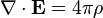$\nabla \cdot \mathbf{E} = 4\pi\rho$	$\nabla \cdot \mathbf{D} = 4\pi\rho_\text{f}$
Gauss's law for magnetism	$\nabla \cdot \mathbf{B} = 0$	same as microscopic
Maxwell–Faraday equation (Faraday's law of induction)	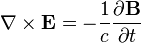$\nabla \times \mathbf{E} = -\frac{1}{c} \frac{\partial \mathbf{B}} {\partial t}$	same as microscopic
Ampère's law (with Maxwell's extension)	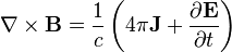$\nabla \times \mathbf{B} = \frac{1}{c} \left(4\pi\mathbf{J} + \frac{\partial \mathbf{E}}{\partial t} \right)$	$\nabla \times \mathbf{H} = \frac{1}{c} \left(4\pi\mathbf{J}_\text{f} + \frac{\partial \mathbf{D}} {\partial t} \right)$

Alternative formulations

For an overview, see Mathematical descriptions of the electromagnetic field.

For the equations in special relativity, see classical electromagnetism and special relativity and covariant formulation of classical electromagnetism.

For the equations in general relativity, see Maxwell's equations in curved spacetime.

For the equations in quantum field theory, see quantum electrodynamics.

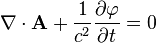
Following is a summary of some of the numerous other ways to write the microscopic Maxwell's equations, showing they can be formulated using different points of view and mathematical formalisms that describe the same physics. Often, they are also called the Maxwell equations. The direct space–time formulations make manifest that the Maxwell equations are relativistically invariant (in fact studying the hidden symmetry of the vector calculus formulation was a major source of inspiration for relativity theory). In addition, the formulation using potentials was originally introduced as a convenient way to solve the equations but with all the observable physics contained in the fields. The potentials play a central role in quantum mechanics, however, and act quantum mechanically with observable consequences even when the fields vanish (Aharonov–Bohm effect). See the main articles for the details of each formulation. SI units are used throughout.

Formalism	Formulation	Homogeneous equations	Non-homogeneous equations
Vector calculus	Fields 3D Euclidean space + time	$\nabla\cdot\mathbf{B}=0$ $\nabla\times\mathbf{E}+\frac{\partial \mathbf{B}}{\partial t}=0$	$\nabla\cdot\mathbf{E}=\frac{\rho}{\varepsilon_0}$ $\nabla\times\mathbf{B}-\frac{1}{c^2}\frac{\partial \mathbf{E}}{\partial t}=\mu_0\mathbf{J}$
	Potentials (any gauge) 3D Euclidean space + time	$\mathbf B = \mathbf \nabla \times \mathbf A$ $\mathbf E = - \mathbf \nabla \varphi - \frac{\partial \mathbf A}{\partial t}$	$\nabla^2 \varphi + \frac{\partial}{\partial t} \left ( \mathbf \nabla \cdot \mathbf A \right ) = - \frac{\rho}{\varepsilon_0}$ $\Box\mathbf A+\mathbf \nabla \left ( \mathbf \nabla \cdot \mathbf A + \frac{1}{c^2} \frac{\partial \varphi}{\partial t} \right ) = \mu_0 \mathbf J$
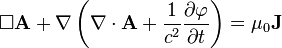
	Potentials (Lorenz gauge) 3D Euclidean space + time	$\mathbf B = \mathbf \nabla \times \mathbf A$ $\mathbf E = - \mathbf \nabla \varphi - \frac{\partial \mathbf A}{\partial t}$ $\mathbf \nabla \cdot \mathbf A + \frac{1}{c^2}\frac{\partial \varphi}{\partial t} = 0$	$\Box \varphi = \frac{\rho}{\varepsilon_0}$ $\Box\mathbf A = \mu_0 \mathbf J$
Tensor calculus	Fields Minkowski space	$\partial_{[\alpha} F_{\beta\gamma]}= 0$	$\partial_\alpha F^{\beta\alpha} = \mu_0 J^\beta$
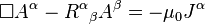
	Potentials (any gauge) Minkowski space	$F_{\alpha\beta} = \partial_{[\alpha} A_{\beta]}$	$\partial_\alpha \partial^{[\beta} A^{\alpha]} = \mu_0 J^\beta$
	Potentials (Lorenz gauge) Minkowski space	$F_{\alpha\beta} = \partial_{[\alpha} A_{\beta]}$ $\partial_\alpha A^\alpha = 0$	$\Box A^\alpha = \mu_0 J^\alpha$
	Fields any space–time	$\partial_{[\alpha} F_{\beta\gamma]}= \nabla_{[\alpha} F_{\beta\gamma]} = 0$	$\nabla_\alpha (\sqrt{-g} F^{\beta\alpha}) = \mu_0 J^\beta$
	Potentials (any gauge) any space–time	$F_{\alpha\beta} = \partial_{[\alpha} A_{\beta]} = \nabla_{[\alpha} A_{\beta]}$	$\nabla_\alpha (\sqrt{-g}\nabla^{[\beta} A^{\alpha]} ) = \mu_0 J^\beta$
	Potentials (Lorenz gauge) any space–time	$F_{\alpha\beta} = \partial_{[\alpha} A_{\beta]} = \nabla_{[\alpha} A_{\beta]},$ $\nabla_\alpha A^{\alpha} = 0$	$\Box A^{\alpha} - R^{\alpha}{}_{\beta} A^\beta = -\mu_0 J^\alpha$
Differential forms	Fields any space–time	$\mathrm{d} F = 0$	$\mathrm{d} {*} F = \mu_0 J$
	Potentials (any gauge) any space–time	$F = \mathrm{d} A$	$\mathrm{d} {*} \mathrm{d} A = \mu_0 J$
	Potentials (Lorenz gauge) any space–time	$F = \mathrm{d} A$ $\mathrm{d} {\star} A = 0$	${\star} \Box A = \mu_0 J$

where

In the vector formulation on Euclidean space + time, $\varphi$ is the electrical potential, $A$ is the vector potential and 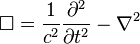$\Box = \frac{1}{c^2} \frac{\partial^2} {\partial t^2}-\nabla^2$ is the D'Alembert operator.
In the tensor calculus formulation, the electromagnetic tensor $F_{\alpha\beta}$ is an antisymmetric covariant rank 2 tensor, the four-potential $A_\alpha$ is a covariant vector, the current $J^\alpha$ is a vector density, the square bracket [ ] denotes antisymmetrization of indices, $\partial_\alpha$ is the derivative with respect to the coordinate $x^\alpha$ . On Minkowski space coordinates are chosen with respect to an inertial frame; $(x^\alpha) = (ct, x, y,z)$ , so that the metric tensor used to raise and lower indices is $\eta_{\alpha\beta} = \mathrm{diag}(1,-1,-1,-1)$ . The D'Alembert operator on Minkowski space is $\Box = \partial_\alpha\partial^\alpha$ as in the vector formulation. On general space–times, the coordinate system $x^\alpha$ is arbitrary, the covariant derivative $\nabla_\alpha$ , the Ricci tensor $R_{\alpha\beta}$ and raising and lowering of indices are defined by the Lorentzian metric $g_{\alpha\beta}$ and the D'Alembert operator is defined as $\Box = \nabla_\alpha\nabla^\alpha$ .
In the differential form formulation on arbitrary space times, $F = F_{\alpha\beta}dx^\alpha\wedge dx^\beta$ is the electromagnetic tensor considered as two form, $A = A_\alpha dx^\alpha$ is the potential 1 form, $J$ is the current (pseudo) 3 form, $\mathrm{d}$ is the exterior derivative, and ${*},{\star}$ are the Hodge stars on forms defined by the Lorentzian metric of space–time (the Hodge star ${*}$ on two forms only depends on the metric up to a local scale i.e. is conformally invariant). The operator $\Box = (-{\star} \mathrm{d} {*} \mathrm{d} - \mathrm{d} {\star} \mathrm{d} {\star})$ is the d'Alembert–Laplace–Beltrami operator on 1-forms on an arbitrary Lorentzian space–time.

Other formulations include the geometric algebra formulation and a matrix representation of Maxwell's equations. Historically, a quaternionic formulation^[8]^[9] was used.

Solutions

Maxwell's equations are partial differential equations that relate the electric and magnetic fields to each other and to the electric charges and currents. Often, the charges and currents are themselves dependent on the electric and magnetic fields via the Lorentz force equation and the constitutive relations. These all form a set of coupled partial differential equations, which are often very difficult to solve. In fact, the solutions of these equations encompass all the diverse phenomena in the entire field of classical electromagnetism. A thorough discussion is far beyond the scope of the article, but some general notes follow.

Like any differential equation, boundary conditions^[10]^[11]^[12] and initial conditions^[13] are necessary for a unique solution. For example, even with no charges and no currents anywhere in spacetime, many solutions to Maxwell's equations are possible, not just the obvious solution $E = B = 0$ . Another solution is $E = constant$ , $B = constant$ , while yet other solutions have electromagnetic waves filling spacetime. In some cases, Maxwell's equations are solved through infinite space, and boundary conditions are given as asymptotic limits at infinity.^[14] In other cases, Maxwell's equations are solved in just a finite region of space, with appropriate boundary conditions on that region: For example, the boundary could be an artificial absorbing boundary representing the rest of the universe,^[15]^[16] or periodic boundary conditions, or (as with a waveguide or cavity resonator) the boundary conditions may describe the walls that isolate a small region from the outside world.^[17]

Jefimenko's equations (or the closely related Liénard–Wiechert potentials) are the explicit solution to Maxwell's equations for the electric and magnetic fields created by any given distribution of charges and currents. It assumes specific initial conditions to obtain the so-called "retarded solution", where the only fields present are the ones created by the charges. Jefimenko's equations are not so helpful in situations when the charges and currents are themselves affected by the fields they create.

Numerical methods for differential equations can be used to approximately solve Maxwell's equations when an exact solution is impossible. These methods usually require a computer, and include the finite element method and finite-difference time-domain method.^[10]^[12]^[18]^[19]^[20] For more details, see Computational electromagnetics.

Maxwell's equations seem overdetermined, in that they involve six unknowns (the three components of $E$ and $B$ ) but eight equations (one for each of the two Gauss's laws, three vector components each for Faraday's and Ampere's laws). (The currents and charges are not unknowns, being freely specifiable subject to charge conservation.) This is related to a certain limited kind of redundancy in Maxwell's equations: It can be proven that any system satisfying Faraday's law and Ampere's law automatically also satisfies the two Gauss's laws, as long as the system's initial condition does.^[21]^[22] Although it is possible to simply ignore the two Gauss's laws in a numerical algorithm (apart from the initial conditions), the imperfect precision of the calculations can lead to ever-increasing violations of those laws. By introducing dummy variables characterizing these violations, the four equations become not overdetermined after all. The resulting formulation can lead to more accurate algorithms that take all four laws into account.^[23]

Limitations for a theory of electromagnetism

While Maxwell's equations (along with the rest of classical electromagnetism) are extraordinarily successful at explaining and predicting a variety of phenomena, they are not exact, but approximations. In some special situations, they can be noticeably inaccurate. Examples include extremely strong fields (see Euler–Heisenberg Lagrangian) and extremely short distances (see vacuum polarization). Moreover, various phenomena occur in the world even though Maxwell's equations predict them to be impossible, such as "nonclassical light" and quantum entanglement of electromagnetic fields (see quantum optics). Finally, any phenomenon involving individual photons, such as the photoelectric effect, Planck's law, the Duane–Hunt law, single-photon light detectors, etc., would be difficult or impossible to explain if Maxwell's equations were exactly true, as Maxwell's equations do not involve photons. For the most accurate predictions in all situations, Maxwell's equations have been superseded by quantum electrodynamics.

Variations

Popular variations on the Maxwell equations as a classical theory of electromagnetic fields are relatively scarce because the standard equations have stood the test of time remarkably well.

Magnetic monopoles

Main article: Magnetic monopole

Maxwell's equations posit that there is electric charge, but no magnetic charge (also called magnetic monopoles), in the universe. Indeed, magnetic charge has never been observed (despite extensive searches)^{[note 4]} and may not exist. If they did exist, both Gauss's law for magnetism and Faraday's law would need to be modified, and the resulting four equations would be fully symmetric under the interchange of electric and magnetic fields.^[24]^[25]

Notes

↑ Maxwell's equations in any form are compatible with relativity. These space-time formulations, though, make that compatibility more readily apparent.
↑ The quantity we would now call $\scriptstyle{1/\sqrt{\mu_0\varepsilon_0}}$ , with units of velocity, was directly measured before Maxwell's equations, in an 1855 experiment by Wilhelm Eduard Weber and Rudolf Kohlrausch. They charged a leyden jar (a kind of capacitor), and measured the electrostatic force associated with the potential; then, they discharged it while measuring the magnetic force from the current in the discharge wire. Their result was 7008310700000000000♠3.107×10⁸ m/s, remarkably close to the speed of light. See The story of electrical and magnetic measurements: from 500 B.C. to the 1940s, by Joseph F. Keithley, p115
↑ In some books—e.g., in U. Krey and A. Owen's Basic Theoretical Physics (Springer 2007)—the term effective charge is used instead of total charge, while free charge is simply called charge.
↑ See magnetic monopole for a discussion of monopole searches. Recently, scientists have discovered that some types of condensed matter, including spin ice and topological insulators, which display emergent behavior resembling magnetic monopoles. (See and .) Although these were described in the popular press as the long-awaited discovery of magnetic monopoles, they are only superficially related. A "true" magnetic monopole is something where $\nabla \cdot B \neq 0$ , whereas in these condensed-matter systems, $\nabla \cdot B = 0$ while only $\nabla \cdot H \neq 0$ .

References

↑ David J Griffiths (1999). Introduction to electrodynamics (Third ed.). Prentice Hall. pp. 559–562. ISBN 0-13-805326-X.
↑ Šolín, Pavel (2006). Partial differential equations and the finite element method. John Wiley and Sons. p. 273. ISBN 0-471-72070-4.
↑ 3.0 3.1 3.2 J.D. Jackson, "Maxwell's Equations" video glossary entry
↑ Principles of physics: a calculus-based text, by R.A. Serway, J.W. Jewett, page 809.
↑ See David J. Griffiths (1999). "4.2.2". Introduction to Electrodynamics (third ed.). Prentice Hall. for a good description of how $P$ relates to the bound charge.
↑ See David J. Griffiths (1999). "6.2.2". Introduction to Electrodynamics (third ed.). Prentice Hall. for a good description of how $M$ relates to the bound current.
↑ Littlejohn, Robert (Fall 2007). "Gaussian, SI and Other Systems of Units in Electromagnetic Theory" (PDF). Physics 221A, University of California, Berkeley lecture notes. Retrieved 2008-05-06.
↑ P.M. Jack (2003). "Physical Space as a Quaternion Structure I: Maxwell Equations. A Brief Note.". Toronto, Canada. arXiv:math-ph/0307038.
↑ A. Waser (2000). "On the Notation of Maxwell's Field Equations" (PDF). AW-Verlag.
↑ 10.0 10.1 Peter Monk (2003). Finite Element Methods for Maxwell's Equations. Oxford UK: Oxford University Press. p. 1 ff. ISBN 0-19-850888-3.
↑ Thomas B. A. Senior & John Leonidas Volakis (1995-03-01). Approximate Boundary Conditions in Electromagnetics. London UK: Institution of Electrical Engineers. p. 261 ff. ISBN 0-85296-849-3.
↑ 12.0 12.1 T Hagstrom (Björn Engquist & Gregory A. Kriegsmann, Eds.) (1997). Computational Wave Propagation. Berlin: Springer. p. 1 ff. ISBN 0-387-94874-0.
↑ Henning F. Harmuth & Malek G. M. Hussain (1994). Propagation of Electromagnetic Signals. Singapore: World Scientific. p. 17. ISBN 981-02-1689-0.
↑ David M Cook (2002). The Theory of the Electromagnetic Field. Mineola NY: Courier Dover Publications. p. 335 ff. ISBN 0-486-42567-3.
↑ Jean-Michel Lourtioz (2005-05-23). Photonic Crystals: Towards Nanoscale Photonic Devices. Berlin: Springer. p. 84. ISBN 3-540-24431-X.
↑ S. G. Johnson, Notes on Perfectly Matched Layers, online MIT course notes (Aug. 2007).
↑ S. F. Mahmoud (1991). Electromagnetic Waveguides: Theory and Applications. London UK: Institution of Electrical Engineers. Chapter 2. ISBN 0-86341-232-7.
↑ John Leonidas Volakis, Arindam Chatterjee & Leo C. Kempel (1998). Finite element method for electromagnetics : antennas, microwave circuits, and scattering applications. New York: Wiley IEEE. p. 79 ff. ISBN 0-7803-3425-6.
↑ Bernard Friedman (1990). Principles and Techniques of Applied Mathematics. Mineola NY: Dover Publications. ISBN 0-486-66444-9.
↑ Taflove A & Hagness S C (2005). Computational Electrodynamics: The Finite-difference Time-domain Method. Boston MA: Artech House. Chapters 6 & 7. ISBN 1-58053-832-0.
↑ H Freistühler & G Warnecke (2001). Hyperbolic Problems: Theory, Numerics, Applications. p. 605.
↑ J Rosen. "Redundancy and superfluity for electromagnetic fields and potentials". American Journal of Physics 48 (12): 1071. Bibcode:1980AmJPh..48.1071R. doi:10.1119/1.12289.
↑ B Jiang & J Wu & L.A. Povinelli (1996). "The Origin of Spurious Solutions in Computational Electromagnetics". Journal of Computational Physics 125 (1): 104. Bibcode:1996JCoPh.125..104J. doi:10.1006/jcph.1996.0082.
↑ J.D. Jackson. "6.11". Classical Electrodynamics (3rd ed.). ISBN 0-471-43132-X.
↑ "IEEEGHN: Maxwell's Equations". Ieeeghn.org. Retrieved 2008-10-19.

Further reading can be found in list of textbooks in electromagnetism

Historical publications

On Faraday's Lines of Force – 1855/56 Maxwell's first paper (Part 1 & 2) – Compiled by Blaze Labs Research (PDF)
On Physical Lines of Force – 1861 Maxwell's 1861 paper describing magnetic lines of Force – Predecessor to 1873 Treatise
James Clerk Maxwell, "A Dynamical Theory of the Electromagnetic Field", Philosophical Transactions of the Royal Society of London 155, 459–512 (1865). (This article accompanied a December 8, 1864 presentation by Maxwell to the Royal Society.)
- A Dynamical Theory Of The Electromagnetic Field – 1865 Maxwell's 1865 paper describing his 20 Equations, link from Google Books.
J. Clerk Maxwell (1873) A Treatise on Electricity and Magnetism
- Maxwell, J.C., A Treatise on Electricity And Magnetism – Volume 1 – 1873 – Posner Memorial Collection – Carnegie Mellon University
- Maxwell, J.C., A Treatise on Electricity And Magnetism – Volume 2 – 1873 – Posner Memorial Collection – Carnegie Mellon University

The developments before relativity:

Joseph Larmor (1897) "On a dynamical theory of the electric and luminiferous medium", Phil. Trans. Roy. Soc. 190, 205–300 (third and last in a series of papers with the same name).
Hendrik Lorentz (1899) "Simplified theory of electrical and optical phenomena in moving systems", Proc. Acad. Science Amsterdam, I, 427–43.
Hendrik Lorentz (1904) "Electromagnetic phenomena in a system moving with any velocity less than that of light", Proc. Acad. Science Amsterdam, IV, 669–78.
Henri Poincaré (1900) "La théorie de Lorentz et le Principe de Réaction", Archives Néerlandaises, V, 253–78.
Henri Poincaré (1902) La Science et l'Hypothèse
Henri Poincaré (1905) "Sur la dynamique de l'électron", Comptes rendus de l'Académie des Sciences, 140, 1504–8.
Catt, Walton and Davidson. "The History of Displacement Current". Wireless World, March 1979.

External links

Hazewinkel, Michiel, ed. (2001), "Maxwell equations", Encyclopedia of Mathematics, Springer, ISBN 978-1-55608-010-4
maxwells-equations.com — An intuitive tutorial of Maxwell's equations.
Mathematical aspects of Maxwell's equation are discussed on the Dispersive PDE Wiki.

Modern treatments

Electromagnetism, B. Crowell, Fullerton College
Lecture series: Relativity and electromagnetism, R. Fitzpatrick, University of Texas at Austin
Electromagnetic waves from Maxwell's equations on Project PHYSNET.
MIT Video Lecture Series (36 x 50 minute lectures) (in .mp4 format) – Electricity and Magnetism Taught by Professor Walter Lewin.

Other

Branches of physics

Divisions	Applied Experimental Theoretical

Energy Motion	Thermodynamics Mechanics Classical Lagrangian Hamiltonian Continuum Celestial Statistical Fluid Quantum

Waves Fields	Gravitation Electromagnetism Quantum field theory Relativity Special General

By speciality	Accelerator Acoustics Astrophysics Nuclear Stellar Heliophysics Solar Space Astroparticle Atomic–molecular–optical (AMO) Computational Condensed matter Solid-state Digital Engineering Material Mathematical Nuclear Optics Geometrical Physical Nonlinear Quantum Particle Phenomenology Plasma Polymer Statistical

Physics with other sciences	Biophysics Cardiophysics Biomechanics Medical Neurophysics Agrophysics Soil Atmospheric physics Chemical Econophysics Geophysics Psychophysics

Relativity

Special
relativity

Background	Principle of relativity Introduction to special relativity Special relativity

Foundations	Relative motion Frame of reference Speed of light Maxwell's equations

Formulation	Galilean relativity Galilean transformation Lorentz transformation

Consequences	Time dilation Relativistic mass Mass–energy equivalence Length contraction Relativity of simultaneity Relativistic Doppler effect Thomas precession Relativistic disks

Spacetime	Minkowski spacetime World line Spacetime diagrams Light cone

General
relativity

Background	Introduction Mathematical formulation Resources

Fundamental concepts	Special relativity Equivalence principle World line Riemannian geometry Minkowski diagram

Phenomena	Two-body problem Lenses Waves Frame-dragging Geodetic effect Event horizon Singularity Black hole

Equations	Linearized gravity Post-Newtonian formalism Einstein field equations Geodesic equation Friedmann equations ADM formalism BSSN formalism Hamilton–Jacobi–Einstein equation

Advanced theories	Kaluza–Klein Quantum gravity Brans–Dicke theory

Solutions	Schwarzschild Reissner–Nordström Gödel Kerr Kerr–Newman Kasner Taub–NUT Milne Robertson–Walker pp-wave van Stockum dust

Scientists

Maxwell's equations

Formulation in terms of electric and magnetic fields

Conventional formulation in SI units

Relationship between differential and integral formulations

Flux and divergence

Circulation and curl

Time evolution

Conceptual descriptions

Gauss's law

Gauss's law for magnetism

Faraday's law

Ampère's law with Maxwell's addition

Vacuum equations, electromagnetic waves and speed of light

"Microscopic" versus "macroscopic"

Bound charge and current

Auxiliary fields, polarization and magnetization

Constitutive relations

Equations in Gaussian units

Alternative formulations

Solutions

Limitations for a theory of electromagnetism

Variations

Magnetic monopoles

See also

Notes

References

Historical publications

External links

Modern treatments

Other