Matthews correlation coefficient
The Matthews correlation coefficient is used in machine learning as a measure of the quality of binary (two-class) classifications, introduced by biochemist Brian W. Matthews in 1975.[1] It takes into account true and false positives and negatives and is generally regarded as a balanced measure which can be used even if the classes are of very different sizes. The MCC is in essence a correlation coefficient between the observed and predicted binary classifications; it returns a value between −1 and +1. A coefficient of +1 represents a perfect prediction, 0 no better than random prediction and −1 indicates total disagreement between prediction and observation. The statistic is also known as the phi coefficient. MCC is related to the chi-square statistic for a 2×2 contingency table
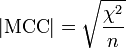
where n is the total number of observations.
While there is no perfect way of describing the confusion matrix of true and false positives and negatives by a single number, the Matthews correlation coefficient is generally regarded as being one of the best such measures. Other measures, such as the proportion of correct predictions (also termed accuracy), are not useful when the two classes are of very different sizes. For example, assigning every object to the larger set achieves a high proportion of correct predictions, but is not generally a useful classification.
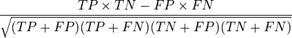
The MCC can be calculated directly from the confusion matrix using the formula:
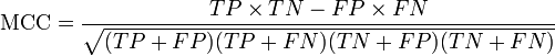
In this equation, TP is the number of true positives, TN the number of true negatives, FP the number of false positives and FN the number of false negatives. If any of the four sums in the denominator is zero, the denominator can be arbitrarily set to one; this results in a Matthews correlation coefficient of zero, which can be shown to be the correct limiting value.
The original formula as given by Matthews was:[1]

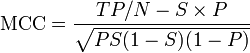
This is equal to the formula given above. As a correlation coefficient, the Matthews correlation coefficient is the geometric mean of the regression coefficients of the problem and its dual. The component regression coefficients of the Matthews correlation coefficient are markedness (deltap) and informedness (deltap').[2][3]
Confusion Matrix
|


Let us define an experiment from P positive instances and N negative instances for some condition. The four outcomes can be formulated in a 2×2 contingency table or confusion matrix, as follows:
| Condition (as determined by "Gold standard") | |||||
| Total population | Condition positive | Condition negative | Prevalence = Σ Condition positive/Σ Total population | ||
| Test outcome |
Test outcome positive |
True positive | False positive (Type I error) |
Positive predictive value (PPV), Precision = Σ True positive/Σ Test outcome positive | False discovery rate (FDR) = Σ False positive/Σ Test outcome positive |
| Test outcome negative |
False negative (Type II error) |
True negative | False omission rate (FOR) = Σ False negative/Σ Test outcome negative | Negative predictive value (NPV) = Σ True negative/Σ Test outcome negative | |
| Accuracy (ACC) = Σ True positive + Σ True negative/Σ Total population | True positive rate (TPR), Sensitivity, Recall = Σ True positive/Σ Condition positive | False positive rate (FPR), Fall-out = Σ False positive/Σ Condition negative | Positive likelihood ratio (LR+) = TPR/FPR | Diagnostic odds ratio (DOR) = LR+/LR− | |
| False negative rate (FNR) = Σ False negative/Σ Condition positive | True negative rate (TNR), Specificity (SPC) = Σ True negative/Σ Condition negative | Negative likelihood ratio (LR−) = FNR/TNR | |||
See also
- Phi coefficient
- F1 score
- Cramér's V, a similar measure of association between nominal variables.
- Cohen's kappa
References
- ↑ 1.0 1.1 Matthews, B. W. (1975). "Comparison of the predicted and observed secondary structure of T4 phage lysozyme". Biochimica et Biophysica Acta (BBA) - Protein Structure 405 (2): 442–451. doi:10.1016/0005-2795(75)90109-9.
- ↑ Perruchet, P.; Peereman, R. (2004). "The exploitation of distributional information in syllable processing". J. Neurolinguistics 17: 97–119. doi:10.1016/s0911-6044(03)00059-9.
- ↑ 3.0 3.1 Powers, David M W (2011). "Evaluation: From Precision, Recall and F-Measure to ROC, Informedness, Markedness & Correlation" (PDF). Journal of Machine Learning Technologies 2 (1): 37–63.
- ↑ Fawcelt, Tom (2006). "An Introduction to ROC Analysis". Pattern Recognition Letters 27 (8): 861 – 874. doi:10.1016/j.patrec.2005.10.010.