Master equation

For the master equation used in quantum physics, see Lindblad equation. For the classical and quantum master equations in quantum field theory, see Batalin–Vilkovisky formalism.

In physics and chemistry and related fields, master equations are used to describe the time-evolution of a system that can be modelled as being in exactly one of countable number of states at any given time, and where switching between states is treated probabilistically. The equations are usually a set of differential equations for the variation over time of the probabilities that the system occupies each of the different states.

Introduction

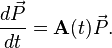
A master equation is a phenomenological set of first-order differential equations describing the time evolution of (usually) the probability of a system to occupy each one of a discrete set of states with regard to a continuous time variable t. The most familiar form of a master equation is a matrix form:

\frac{d\vec{P}}{dt}=\mathbf{A}\vec{P},

where $\vec{P}$ is a column vector (where element i represents state i), and $\mathbf{A}$ is the matrix of connections. The way connections among states are made determines the dimension of the problem; it is either

a d-dimensional system (where d is 1,2,3,...), where any state is connected with exactly its 2d nearest neighbors, or
a network, where every pair of states may have a connection (depending on the network's properties).

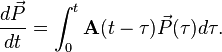
When the connections are time-independent rate constants, the master equation represents a kinetic scheme, and the process is Markovian (any jumping time probability density function for state i is an exponential, with a rate equal to the value of the connection). When the connections depend on the actual time (i.e. matrix $\mathbf{A}$ depends on the time, $\mathbf{A}\rightarrow\mathbf{A}(t)$ ), the process is not stationary and the master equation reads

\frac{d\vec{P}}{dt}=\mathbf{A}(t)\vec{P}.

When the connections represent multi exponential jumping time probability density functions, the process is semi-Markovian, and the equation of motion is an integro-differential equation termed the generalized master equation:

\frac{d\vec{P}}{dt}= \int^t_0 \mathbf{A}(t- \tau )\vec{P}( \tau )d \tau .

The matrix $\mathbf{A}$ can also represent birth and death, meaning that probability is injected (birth) or taken from (death) the system, where then, the process is not in equilibrium.

Detailed description of the matrix $\mathbf{A}$ , and properties of the system

Let $\mathbf{A}$ be the matrix describing the transition rates (also known as kinetic rates or reaction rates). As always, the first subscript represents the row, the second subscript the column. That is, the source is given by the second subscript, and the destination by the first subscript. This is the opposite of what one might expect, but it is technically convenient.

For each state k, the increase in occupation probability depends on the contribution from all other states to k, and is given by:

\sum_\ell A_{k\ell}P_\ell,

where $P_\ell,$ is the probability for the system to be in the state $\ell$ , while the matrix $\mathbf{A}$ is filled with a grid of transition-rate constants. Similarly, $P_k$ contributes to the occupation of all other states $P_\ell,$

\sum_\ell A_{\ell k}P_k,

In probability theory, this identifies the evolution as a continuous-time Markov process, with the integrated master equation obeying a Chapman–Kolmogorov equation.

The master equation can be simplified so that the terms with ℓ = k do not appear in the summation. This allows calculations even if the main diagonal of the $\mathbf{A}$ is not defined or has been assigned an arbitrary value.

\frac{dP_k}{dt} =\sum_\ell(A_{k\ell}P_\ell) =\sum_{\ell\neq k}(A_{k\ell}P_\ell) + A_{kk}P_k =\sum_{\ell\neq k}(A_{k\ell}P_\ell - A_{\ell k}P_k).

The final equality arises from the fact that

\sum_\ell(A_{\ell k}) = 0

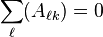
and so

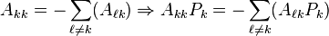A_{kk} = -\sum_{\ell\neq k}(A_{\ell k}) \Rightarrow A_{kk} P_k = -\sum_{\ell\neq k}(A_{\ell k} P_k)

The master equation exhibits detailed balance if each of the terms of the summation disappears separately at equilibrium — i.e. if, for all states k and ℓ having equilibrium probabilities $\scriptstyle\pi_k$ and $\scriptstyle\pi_\ell$ ,

A_{k \ell} \pi_\ell = A_{\ell k} \pi_k .

These symmetry relations were proved on the basis of the time reversibility of microscopic dynamics (microscopic reversibility) as Onsager reciprocal relations.

Examples of master equations

Many physical problems in classical, quantum mechanics and problems in other sciences, can be reduced to the form of a master equation, thereby performing a great simplification of the problem (see mathematical model).

The Lindblad equation in quantum mechanics is a generalization of the master equation describing the time evolution of a density matrix. Though the Lindblad equation is often referred to as a master equation, it is not one in the usual sense, as it governs not only the time evolution of probabilities (diagonal elements of the density matrix), but also of variables containing information about quantum coherence between the states of the system (non-diagonal elements of the density matrix).

Another special case of the master equation is the Fokker-Planck equation which describes the time evolution of a continuous probability distribution. Complicated master equations which resist analytic treatment can be cast into this form (under various approximations), by using approximation techniques such as the system size expansion.

Quantum master equations

A quantum master equation is a generalization of the idea of a master equation. Rather than just a system of differential equations for a set of probabilities (which only constitutes the diagonal elements of a density matrix), quantum master equations are differential equations for the entire density matrix, including off-diagonal elements. A density matrix with only diagonal elements can be modeled as a classical random process, therefore such an "ordinary" master equation is considered classical. Off-diagonal elements represent quantum coherence which is a physical characteristic that is intrinsically quantum mechanical.

The Lindblad equation was a primitive example of a quantum master equation. More accurate quantum master equations include the polaron transformed quantum master equation, and the variational polaron transformed quantum master equation.^[1]

References

↑ McCutcheon, D.; N. S. Dattani, E. Gauger, B. Lovett, A. Nazir (25 August 2011). "A general approach to quantum dynamics using a variational master equation: Application to phonon-damped Rabi rotations in quantum dots". Physical Review B Rapid Communications 84: 081305R. doi:10.1103/PhysRevB.84.081305.

van Kampen, N. G. (1981). Stochastic processes in physics and chemistry. North Holland. ISBN 978-0-444-52965-7.

Gardiner, C. W. (1985). Handbook of Stochastic Methods. Springer. ISBN 3-540-20882-8.
Risken, H. (1984). The Fokker-Planck Equation. Springer. ISBN 3-540-61530-X.

External links

Timothy Jones, A Quantum Optics Derivation (2006)