Marsaglia polar method

The polar method (attributed to George Marsaglia, 1964^[1]) is a pseudo-random number sampling method for generating a pair of independent standard normal random variables.^[2] While it is superior to the Box–Muller transform,^[3] the Ziggurat algorithm is even more efficient.^[4]

Standard normal random variables are frequently used in computer science, computational statistics, and in particular, in applications of the Monte Carlo method.

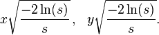
The polar method works by choosing random points (x, y) in the square −1 < x < 1, −1 < y < 1 until

and then returning the required pair of normal random variables as

Theoretical basis

The underlying theory may be summarized as follows:

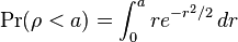
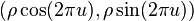
If u is uniformly distributed in the interval 0 ≤ u < 1, then the point (cos(2πu), sin(2πu)) is uniformly distributed on the unit circumference x² + y² = 1, and multiplying that point by an independent random variable ρ whose distribution is

will produce a point

whose coordinates are jointly distributed as two independent standard normal random variables.

History

This idea dates back to Laplace, whom Gauss credits with finding the above

by taking the square root of

The transformation to polar coordinates makes evident that θ is uniformly distributed (constant density) from 0 to 2π, and that the radial distance r has density

(r² has the appropriate chi square distribution.)

This method of producing a pair of independent standard normal variates by radially projecting a random point on the unit circumference to a distance given by the square root of a chi-square-2 variate is called the polar method for generating a pair of normal random variables,

Practical considerations

A direct application of this idea,

is called the Box Muller transform, in which the chi variate is usually generated as

but that transform requires logarithm, square root, sine and cosine functions. On some processors, the cosine and sine of the same argument can be calculated in parallel using a single instruction.^[5] Notably for Intel based machines, one can use fsincos assembler instruction or the expi instruction (available e.g. in D), to calculate complex

and just separate the real and imaginary parts.

The polar method, in which a random point (x, y) inside the unit circle is projected onto the unit circumference by setting s = x² + y² and forming the point

is a faster procedure. Some researchers argue that the conditional if instruction (for rejecting a point outside of the unit circle), can make programs slower on modern processors equipped with pipelining and branch prediction.^[6] Also this procedure requires about 21% more evaluations of the underlying random number generator (only of generated points lie inside of unit circle).

That random point on the circumference is then radially projected the required random distance by means of

using the same s because that s is independent of the random point on the circumference and is itself uniformly distributed from 0 to 1.

Implementation

Simple implementation in Java using the mean and standard deviation:

private static double spare;
private static boolean isSpareReady = false;
 
public static synchronized double getGaussian(double mean, double stdDev) {
    if (isSpareReady) {
        isSpareReady = false;
        return spare * stdDev + mean;
    } else {
        double u, v, s;
        do {
            u = Math.random() * 2 - 1;
            v = Math.random() * 2 - 1;
            s = u * u + v * v;
        } while (s >= 1 || s == 0);
        double mul = Math.sqrt(-2.0 * Math.log(s) / s);
        spare = v * mul;
        isSpareReady = true;
        return mean + stdDev * u * mul;
    }
}

An implementation in C++ using the variance:

double generateGaussianNoise(const double &variance)
{
	static bool hasSpare = false;
	static double spare;
 
	if(hasSpare)
	{
		hasSpare = false;
		return variance * spare;
	}
 
	hasSpare = true;
	static qreal u, v, s;
	do
	{
		u = (rand() / ((double) RAND_MAX)) * 2 - 1;
		v = (rand() / ((double) RAND_MAX)) * 2 - 1;
		s = u * u + v * v;
	}
	while(s >= 1 || s == 0);
 
	s = sqrt(-2.0 * log(s) / s);
	spare = v * s;
	return variance * u * s;
}

References

- ↑ A convenient method for generating normal variables, G. Marsaglia and T. A. Bray, SIAM Rev. 6, 260–264, 1964
- ↑ Peter E. Kloeden Eckhard Platen Henri Schurz, Numerical Solution of SDE Through Computer Experiments, Springer, 1994.
- ↑ Glasserman, Paul (2004), Monte Carlo Methods in Financial Engineering, Applications of Mathematics: Stochastic Modelling and Applied Probability 53, Springer, p. 66, ISBN 9780387004518.
- ↑ http://doi.acm.org/10.1145/1287620.1287622 Gaussian Random Number Generators, D. Thomas and W. Luk and P. Leong and J. Villasenor, ACM Computing Surveys, Vol. 39(4), Article 11, 2007, doi:10.1145/1287620.1287622
- ↑ Kanter, David. "Intel’s Ivy Bridge Graphics Architecture". Real World Tech. Retrieved 8 April 2013.
- ↑ This effect can be heightened in a GPU generating many variates in parallel, where a rejection on one processor can slow down many other processors. See section 7 of Thomas, David B.; Howes, Lee W.; Luk, Wayne (2009), "A comparison of CPUs, GPUs, FPGAs, and massively parallel processor arrays for random number generation", in Chow, Paul; Cheung, Peter Y. K., Proceedings of the ACM/SIGDA 17th International Symposium on Field Programmable Gate Arrays, FPGA 2009, Monterey, California, USA, February 22-24, 2009, Association for Computing Machinery, pp. 63–72, doi:10.1145/1508128.1508139.