Magnetohydrodynamic turbulence
Magnetohydrodynamics (MHD) deals with what is a quasi-neutral fluid with very high conductivity. The fluid approximation implies that we focus on macro length and time scales which are much larger than the collision length and collision time respectively. In this article we will discuss MHD turbulence which is observed when the Reynolds number of the magnetofluid is large.
Incompressible MHD equations
The incompressible MHD equations are
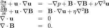
where u, B, p represent the velocity, magnetic, and total pressure (thermal+magnetic) fields,  and
and  represent kinematic viscosity and magnetic diffusivity. The third equation is the incompressibility condition. In the above equation, the magnetic field is in Alfvén units (same as velocity units).
The total magnetic field can be split into two parts:  (mean + fluctuations).
The above equations in terms of Elsässer variables ( ) are
) are

where  . Nonlinear interactions occur between the Alfvénic fluctuations
  .
.
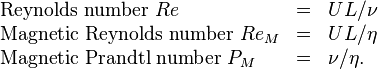
The important nondimensional parameters for MHD are
The magnetic Prandtl number is an important property of the fluid. Liquid metals have small magnetic Prandtl numbers, for example, liquid sodium's  is around
  . But plasmas have large .
The Reynolds number is the ratio of the nonlinear term  of the Navier-Stokes equation to the viscous term. While the magnetic Reynolds number is the ratio of the nonlinear term and the diffusive term of the induction equation.
In many practical situations, the Reynolds number  of the flow is quite large. For such flows typically the velocity and the magnetic fields are random. Such flows are called to exhibit MHD turbulence. Note that
  need not be large for MHD turbulence. plays an important role in dynamo (magnetic field generation) problem.
The mean magnetic field plays an important role in MHD turbulence, for example it can make the turbulence anisotropic; suppress the turbulence by decreasing energy cascade etc. The earlier MHD turbulence models assumed isotropy of turbulence, while the later models have studied anisotropic aspects. In the following discussions will summarize these models. More discussions on MHD turbulence can be found in Biskamp[1] and Verma.[2]
Isotropic models
Iroshnikov[3] and Kraichnan[4] formulated the first phenomenological theory of MHD turbulence. They argued that in the presence
of a strong mean magnetic field,  and
and  wavepackets travel in opposite directions with
the phase velocity of
wavepackets travel in opposite directions with
the phase velocity of  , and interact weakly. The relevant time scale is Alfven time
  . As a results the energy spectra is

where  is the energy cascade rate.
Later Dobrowolny et al.[5] derived the following generalized formulas for the cascade rates of  variables:

where  are the interaction time scales of variables.
Iroshnikov and Kraichnan's phenomenology follows once we choose 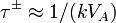 .
.
Marsch[6] chose the nonlinear time scale 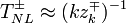 as the interaction time scale for the eddies and derived Kolmogorov-like energy spectrum for the Elsasser variables:

where  and
and  are the energy cascade rates of and respectively, and
  are constants.
Matthaeus and Zhou[7] attempted to combine the above two time scales by postulating the interaction time to be the harmonic mean of Alfven time and nonlinear time.
The main difference between the two competing phenomenologies (-3/2 and -5/3) is the chosen time scales for the interaction time. The main underlying assumption in that Iroshnikov and Kraichnan's phenomenology should work for strong mean magnetic field, whereas Marsh's phenomenology should work when the fluctuations dominate the mean magnetic field (strong turbulence).
However, as we will discuss below, the solar wind observations and numerical simulations tend to favour -5/3 energy spectrum
even when the mean magnetic field is stronger compared to the fluctuations. This issue was resolved by Verma[8] using renormalization group analysis by showing that the Alfvénic fluctuations are affected by scale-dependent "local mean magnetic field". The local mean magnetic field scales as  , substitution of which in Dobrowolny's equation yields Kolmogorov's energy spectrum for MHD turbulence.
Renormalization group analysis have been also performed for computing the renormalized viscosity and resistivity. It was shown that these diffusive quantities scale as  that again yields
  energy spectra consistent with Kolmogorov-like model for MHD turbulence. The above renormalization group calculation has been performed for both zero and nonzero cross helicity.
The above phenomenologies assume isotropic turbulence that is not the case in the presence of a mean magnetic field. The mean magnetic field typically suppresses the energy cascade along the direction of the mean magnetic field.[9]
Anisotropic models
Mean magnetic field makes turbulence anisotropic. This aspect has been studied in last two decades. In the limit
 , Galtier et al.[10] showed using kinetic equations that
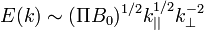
where  and
and  are components of the wavenumber parallel and perpendicular to mean magnetic field. The above limit is called the weak turbulence limit.
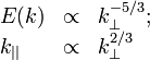
Under the strong turbulence limit,  , Goldereich and Sridhar[11] argue that
  ("critical balanced state") which implies that
The above anisotropic turbulence phenomenology has been extended for large cross helicity MHD.
Solar wind observations
Solar wind plasma is in turbulent state. Researchers have calculated the energy spectra of the solar wind plasma from the data
collected from the spacecraft. The kinetic and magnetic energy spectra, as well as  are closer to
compared to
are closer to
compared to  , thus favoring Kolmogorov-like phenomenology for MHD
turbulence.[12][13] The interplanetary and interstellar electron density fluctuations also provide
a window for investigating MHD turbulence.
, thus favoring Kolmogorov-like phenomenology for MHD
turbulence.[12][13] The interplanetary and interstellar electron density fluctuations also provide
a window for investigating MHD turbulence.
Numerical simulations
The theoretical models discussed above are tested using the high resolution direct numerical simulation (DNS). Number of recent simulations report the spectral indices to be closer to 5/3.[14] There are others that report the spectral indices near 3/2. The regime of power law is typically less than a decade. Since 5/3 and 3/2 are quite close numerically, it is quite difficult to ascertain the validity of MHD turbulence models from the energy spectra.
Energy fluxes  can be more reliable quantities to validate MHD turbulence models.
When
can be more reliable quantities to validate MHD turbulence models.
When 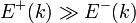 (high cross helicity fluid or imbalanced MHD) the energy flux predictions of Kraichnan and Iroshnikov model is very different from that of Kolmogorov-like model. It has been shown using DNS that the fluxes computed from the numerical simulations are in better agreement with Kolmogorov-like model compared to Kraichnan and Iroshnikov model.[15]
Anisotropic aspects of MHD turbulence have also been studied using numerical simulations. The predictions of Goldreich and Sridhar[11] ( ) have been verified in many simulations. Some of the recent simulations report dynamic alignment of velocity and magnetic field fluctuations in the inertial range, and energy spectra.[16]
Energy transfer
Energy transfer among various scales between the velocity and magnetic field is an important problem in MHD turbulence. These quantities have been computed both theoretically and numerically.[2] These calculations show a significant energy transfer from the large scale velocity field to the large scale magnetic field. Also, the cascade of magnetic energy is typically forward. These results have critical bearing on dynamo problem.
There are many open challenges in this field that hopefully will be resolved in near future with the help of numerical simulations, theoretical modelling, experiments, and observations (e.g., solar wind).
See also
- Magnetohydrodynamics
- Turbulence
- Alfvén wave
- Solar dynamo
- Reynolds number
- Navier–Stokes equations
- Computational magnetohydrodynamics
- Computational fluid dynamics
- Solar wind
- Magnetic flow meter
- Ionic liquid
- List of plasma (physics) articles
References
- ↑ D. Biskamp (2003), Magnetohydrodynamical Turbulence, (Cambridge University Press, Cambridge.)
- ↑ 2.0 2.1 M. K. Verma (2004), Statistical theory of magnetohydrodynamic turbulence, Phys. Rep., 401, 229.
- ↑ P. S. Iroshnikov (1964), Turbulence of a Conducting Fluid in a Strong Magnetic Field, Soviet Astronomy, 7, 566.
- ↑ R. Kraichnan(1965), Inertial-Range Spectrum of Hydromagnetic Turbulence, Physics of Fluids, 8, 1385.
- ↑ M. Dobrowlny, A. Mangeney, P. Veltri (1980), Fully developed anisotropic hydromagnetic turbulence in interplanetary plasma, Phys. Rev. Lett., 45, 144.
- ↑ E. Marsch (1990), Turbulence in the solar wind, in: G. Klare (Ed.), Reviews in Modern Astronomy, Springer, Berlin, p. 43.
- ↑ W. H. Matthaeus, Y. Zhou (1989), Extended inertial range phenomenology of magnetohydrodynamic turbulence, Phys. Fluids B, 1, 1929.
- ↑ M. K. Verma (1999), Mean magnetic field renormalization and Kolmogorov’s energy spectrum in magnetohydrodynamic turbulence, Phys. Plasmas 6, 1455.
- ↑ J. V. Shebalin, W. H. Matthaeus, D. Montgomery (1983), Anisotropy in mhd turbulence due to a mean magnetic field, J. Plasma Phys., 29, 525.
- ↑ S. Galtier, S. V. Nazarenko, A. C. Newell, A. Pouquet (2000), A weak turbulence theory for incompressible magnetohydrodynamics, Journal of Plasma Physics, 63, 447
- ↑ 11.0 11.1 Goldreich, P. & Sridhar, S. (1995), Toward a theory of interstellar turbulence. 2: Strong Alfvénic turbulence, Astrophysical Journal, 438, 763
- ↑ W. H. Matthaeus, M. L. Goldstein (1982), Measurement of the rugged invariants of magnetohydrodynamic turbulence in the solar wind, J. Geophys. Res., 87, 6011.
- ↑ D. A. Roberts, M. L. Goldstein (1991), Turbulence and waves in the solar wind, Rev. Geophys., 29, 932.
- ↑ W.-C. Müller, D. Biskamp (2000) , Scaling properties of three-dimensional magnetohydrodynamic turbulence, Phys. Rev. Lett., 84, 475.
- ↑ M. K. Verma, D. A. Roberts, M. L. Goldstein, S. Ghosh, W. T. Stribling (1996), A numerical study of the nonlinear cascade of energy in magnetohydrodynamic turbulence, J. Geophys. Res., 101, 21619.
- ↑ J. Mason, F. Cattaneo, S. Boldyrev (2008), Numerical measurements of the spectrum in magnetohydrodynamic turbulence, Phys. Rev. E, 77, 036403.