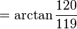
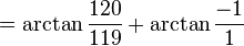
Machin-like formula

In mathematics, Machin-like formulae are a popular technique for computing π to a large number of digits. They are generalizations of John Machin's formula from 1706:

\frac{\pi}{4} = 4 \arctan \frac{1}{5} - \arctan \frac{1}{239}

which he used to compute π to 100 decimal places.

Machin-like formulas have the form:

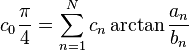
$c_0 \frac{\pi}{4} = \sum_{n=1}^N c_n \arctan \frac{a_n}{b_n}$

(1)

Where $a_n$ and $b_n$ are positive integers such that $a_n < b_n$ , $c_n$ is a signed non-zero integer, and $c_0$ is a positive integer.

These formulae are used in conjunction with the Taylor series expansion for arctangent:

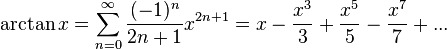
$\arctan x = \sum^{\infin}_{n=0} \frac{(-1)^n}{2n+1} x^{2n+1} = x - \frac{x^3}{3} + \frac{x^5}{5} - \frac{x^7}{7} + ...$

(4)

Derivation

In Angle addition formula we learned the following equations:

\sin(\alpha + \beta) = \sin \alpha \cos \beta + \cos \alpha \sin \beta

\cos(\alpha + \beta) = \cos \alpha \cos \beta - \sin \alpha \sin \beta

Simple algebraic manipulations of these equations yield the following:

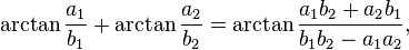
$\arctan \frac{a_1}{b_1} + \arctan \frac{a_2}{b_2} = \arctan\frac{a_1 b_2 + a_2 b_1}{b_1 b_2 - a_1 a_2},$

(2)

$-\frac{\pi}{2} < \arctan \frac{a_1}{b_1} + \arctan \frac{a_2}{b_2} < \frac{\pi}{2}.$

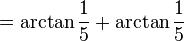
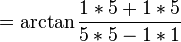
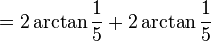
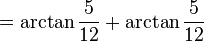
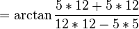
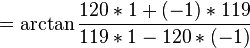
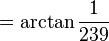
All of the Machin-like formulae can be derived by repeated application of this equation. As an example, we show the derivation of Machin's original formula:

2 \arctan \frac{1}{5}

= \arctan \frac{1}{5} + \arctan \frac{1}{5}

= \arctan \frac {1*5 + 1*5}{5*5 - 1*1}

= \arctan \frac {10}{24}

= \arctan \frac {5}{12}

4 \arctan \frac{1}{5}

= 2 \arctan \frac{1}{5} + 2 \arctan \frac{1}{5}

= \arctan \frac{5}{12} + \arctan \frac{5}{12}

= \arctan \frac{5*12 + 5*12}{12*12 - 5*5}

= \arctan \frac{120}{119}

4 \arctan \frac{1}{5} - \frac{\pi}{4}

= 4 \arctan \frac{1}{5} - \arctan \frac{1}{1}

= 4 \arctan \frac{1}{5} + \arctan \frac{-1}{1}

= \arctan \frac{120}{119} + \arctan \frac{-1}{1}

= \arctan \frac{120*1 + (-1)*119}{119*1 - 120*(-1)}

= \arctan \frac{1}{239}

\frac{\pi}{4} = 4 \arctan \frac{1}{5} - \arctan \frac{1}{239}

An insightful way to visualize equation 2 is to picture what happens when two complex numbers are multiplied together:

(b_1 + a_1 i)*(b_2 + a_2 i)

=b_1 b_2 + a_2 b_1 i + a_1 b_2 i - a_1 a_2

$=(b_1 b_2 - a_1 a_2) + (a_1 b_2 + a_2 b_1) * i$

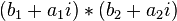
(3)

The angle associated with a complex number $(b_n + a_n i)$ is given by:

\arctan \frac {a_n}{b_n}

Thus, in equation 3, the angle associated with the product is:

\arctan \frac{a_1 b_2 + a_2 b_1}{b_1 b_2 - a_1 a_2}

Note that this is the same expression as occurs in equation 2. Thus equation 2 can be interpreted as saying that the act of multiplying two complex numbers is equivalent to adding their associated angles (see multiplication of complex numbers).

The expression:

c_n \arctan \frac{a_n}{b_n}

is the angle associated with:

(b_n + a_n i)^{c_n}

Equation 1 can be re-written as:

k * (1 + i)^{c_0} = \prod_{n=1}^N (b_n + a_n i)^{c_n}

Where $k$ is an arbitrary constant that accounts for the difference in magnitude between the vectors on the two sides of the equation. The magnitudes can be ignored, only the angles are significant.

Using Complex Numbers

Other formulas may be generated using complex numbers. For example the angle of a complex number $(a + bi)$ is given by $\arctan\frac{b}{a}$ and when you multiply complex numbers you add their angles. If a=b then $\arctan\frac{b}{a}$ is 45 degrees or $\frac{\pi}{4}$ . This means that if the real part and complex part are equal then the arctangent will equal $\frac{\pi}{4}$ . Since the arctangent of one has a very slow convergence rate if we find two complex numbers that when multiplied will result in the same real and imaginary part we will have a Machin-like formula. An example is $(2 + i)$ and $(3 + i)$ . If we multiply these out we will get $(5 + 5i)$ . 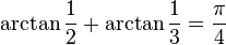Therefore $\arctan\frac{1}{2} + \arctan\frac{1}{3} = \frac{\pi}{4}$ .

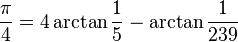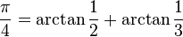
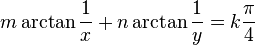
If you want to use complex numbers to show that $\frac{\pi}{4} = 4\arctan\frac{1}{5} - \arctan\frac{1}{239}$ you first must know that when multiplying angles you put the complex number to the power of the number that you are multiplying by. So $(5+i)^4 (-239+i) = -2^2(13^4)(1+i)$ and since the real part and imaginary part are equal then, $4\arctan\frac{1}{5} - \arctan\frac{1}{239} = \frac{\pi}{4}$

Two-term formulas

In the special case where $a_n$ is one, there are exactly four solutions having only two terms.^[1] These are Euler's:

\frac{\pi}{4} = \arctan\frac{1}{2} + \arctan\frac{1}{3}

Hermann's:

\frac{\pi}{4} = 2 \arctan\frac{1}{2} - \arctan\frac{1}{7}

Hutton's (or Vega's^[1]):

\frac{\pi}{4} = 2 \arctan\frac{1}{3} + \arctan\frac{1}{7}

and Machin's:

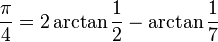
\frac{\pi}{4} = 4 \arctan\frac{1}{5} - \arctan\frac{1}{239}

In the general case, where the value of $a_n$ is not restricted, there are countless other solutions. Example:

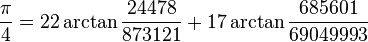
$\frac{\pi}{4} = 22 \arctan\frac{24478}{873121} + 17 \arctan\frac{685601}{69049993}$

(5)

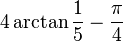
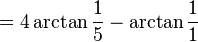
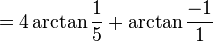
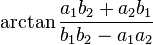
Example

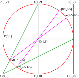
The adjacent diagram demonstrates the relationship between the arctangents and their areas. From the diagram, we have the following:

\begin{align} {\rm area}(PON)&={\rm area}(MOF)=\pi\times\frac{\angle MOF}{2\pi}=\angle MEF=\arctan{1\over2}\\ {\rm area}(POM)&={\rm area}(NOF)=\arctan{1\over3}\\ {\rm area}(POF)&={\pi\over4}=\arctan{1\over2}+\arctan{1\over3}\\ {\rm area}(MON)&=\arctan{1\over7}\\ \arctan{1\over2}&=\arctan{1\over3}+\arctan{1\over7}\end{align}

More terms

The 2002 record for digits of π, 1,241,100,000,000, was obtained by Yasumasa Kanada of Tokyo University. The Calculation was performed on a 64-node Hitachi supercomputer with 1 terabyte of main memory, performing 2 trillion operations per second. The following two equations were both used:

\frac{\pi}{4} = 12 \arctan\frac{1}{49} + 32 \arctan\frac{1}{57} - 5 \arctan\frac{1}{239} + 12 \arctan\frac{1}{110443}

Kikuo Takano (1982).

\frac{\pi}{4} = 44 \arctan\frac{1}{57} + 7 \arctan\frac{1}{239} - 12 \arctan\frac{1}{682} + 24 \arctan\frac{1}{12943}

F. C. M. Störmer (1896).

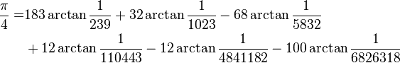
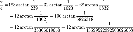
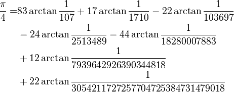
The most efficient currently known Machin-like formulas for computing π:

\begin{align} \frac{\pi}{4} =& 183\arctan\frac{1}{239} + 32\arctan\frac{1}{1023} - 68\arctan\frac{1}{5832}\\ & + 12\arctan\frac{1}{110443} - 12\arctan\frac{1}{4841182} - 100\arctan\frac{1}{6826318}\\ \end{align}

黃見利 (Hwang Chien-Lih) (1997).

\begin{align} \frac{\pi}{4} =& 183\arctan\frac{1}{239} + 32\arctan\frac{1}{1023} - 68\arctan\frac{1}{5832}\\ & + 12\arctan\frac{1}{113021} - 100\arctan\frac{1}{6826318}\\ & - 12\arctan\frac{1}{33366019650} + 12\arctan\frac{1}{43599522992503626068}\\ \end{align}

黃見利 (Hwang Chien-Lih) (2003).

\begin{align} \frac{\pi}{4} =& 83\arctan\frac{1}{107} + 17\arctan\frac{1}{1710} - 22\arctan\frac{1}{103697}\\ & - 24\arctan\frac{1}{2513489} - 44\arctan\frac{1}{18280007883}\\ & + 12\arctan\frac{1}{7939642926390344818}\\ & + 22\arctan\frac{1}{3054211727257704725384731479018}\\ \end{align}

(M.Wetherfield) (2004).

Efficiency

It is not the goal of this section to estimate the actual run time of any given algorithm. Instead, the intention is merely to devise a relative metric by which two algorithms can be compared against each other.

Let $N_d$ be the number of digits to which $\pi$ is to be calculated.

Let $N_t$ be the number of terms in the Taylor series (see equation 4).

Let $u_n$ be the amount of time spent on each digit (for each term in the Taylor series).

The Taylor series will converge when:

\left(\left(\frac{b_n}{a_n}\right)^2\right)^{N_t} = 10^{N_d}

Thus:

N_t = N_d \quad \frac{\ln 10}{2 \ln \frac{b_n}{a_n}}

For the first term in the Taylor series, all $N_d$ digits must be processed. In the last term of the Taylor series, however, there's only one digit remaining to be processed. In all of the intervening terms, the number of digits to be processed can be approximated by linear interpolation. Thus the total is given by:

\frac{N_d N_t}{2}

The run time is given by:

time = \frac{u_n N_d N_t}{2}

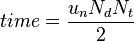
Combining equations, the run time is given by:

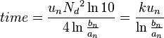
time = \frac{u_n {N_d}^2 \ln 10}{4 \ln \frac{b_n}{a_n}} = \frac{k u_n}{\ln \frac{b_n}{a_n}}

Where $k$ is a constant that combines all of the other constants. Since this is a relative metric, the value of $k$ can be ignored.

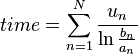
The total time, across all the terms of equation 1, is given by:

time = \sum_{n=1}^N \frac{u_n}{\ln \frac{b_n}{a_n}}

$u_n$ cannot be modelled accurately without detailed knowledge of the specific software. Regardless, we present one possible model.

The software spends most of its time evaluating the Taylor series from equation 4. The primary loop can be summarized in the following pseudo code:

1: \quad term \quad *= \quad {a_n}^2

2: \quad term \quad /= \quad -{b_n}^2

3: \quad tmp \quad = \quad term \quad / \quad (2*n+1)

4: \quad sum \quad += \quad tmp

In this particular model, it is assumed that each of these steps takes approximately the same amount of time. Depending on the software used, this may be a very good approximation or it may be a poor one.

The unit of time is defined such that one step of the pseudo code corresponds to one unit. To execute the loop, in its entirety, requires four units of time. $u_n$ is defined to be four.

Note, however, that if $a_n$ is equal to one, then step one can be skipped. The loop only takes three units of time. $u_n$ is defined to be three.

As an example, consider the equation:

$\frac{\pi}{4} = 44 \arctan \frac{74684}{14967113} + 139 \arctan \frac{1}{239} - 12 \arctan \frac{20138}{15351991}$

(6)

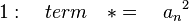
The following table shows the estimated time for each of the terms:

$a_n$	$b_n$	$\frac{b_n}{a_n}$	$\ln \frac{b_n}{a_n}$	$u_n$	$time$
74684	14967113	200.41	5.3003	4	0.75467
1	239	239.00	5.4765	3	0.54780
20138	15351991	762.34	6.6364	4	0.60274

The total time is 0.75467 + 0.54780 + 0.60274 = 1.9052

Compare this with equation 5. The following table shows the estimated time for each of the terms:

$a_n$	$b_n$	$\frac{b_n}{a_n}$	$\ln \frac{b_n}{a_n}$	$u_n$	$time$
24478	873121	35.670	3.5743	4	1.1191
685601	69049993	100.71	4.6123	4	0.8672

The total time is 1.1191 + 0.8672 = 1.9863

The conclusion, based on this particular model, is that equation 6 is slightly faster than equation 5, regardless of the fact that equation 6 has more term(s). This result is typical of the general trend. The dominant factor is the ratio between $a_n$ and $b_n$ . In order to achieve a high ratio, it is necessary to add additional terms. Often, there's a net savings in time.

References

↑ 1.0 1.1 Carl Størmer (1899). $m \arctan\frac{1}{x} + n \arctan\frac{1}{y} = k \frac{\pi}{4}$ . Bulletin de la S.M.F. (in French) 27: 160–170.

External links

Weisstein, Eric W., "Machin-like formulas", MathWorld.
The constant π
Machin's Merit at MathPages
Archimedes' constant pi - Machin's formula gives a proof for the John Machin`s formula